

ABSTRACT
A three-dimensional magnetohydrodynamic (MHD) model for the propagation and dissipation of Alfvén waves in a coronal loop is developed. The model includes the lower atmospheres at the two ends of the loop. The waves originate on small spatial scales (less than 100 km) inside the kilogauss flux elements in the photosphere. The model describes the nonlinear interactions between Alfvén waves using the reduced MHD approximation. The increase of Alfvén speed with height in the chromosphere and transition region (TR) causes strong wave reflection, which leads to counter-propagating waves and turbulence in the photospheric and chromospheric parts of the flux tube. Part of the wave energy is transmitted through the TR and produces turbulence in the corona. We find that the hot coronal loops typically found in active regions can be explained in terms of Alfvén wave turbulence, provided that the small-scale footpoint motions have velocities of 1–2 km s−1 and timescales of 60–200 s. The heating rate per unit volume in the chromosphere is two to three orders of magnitude larger than that in the corona. We construct a series of models with different values of the model parameters, and find that the coronal heating rate increases with coronal field strength and decreases with loop length. We conclude that coronal loops and the underlying chromosphere may both be heated by Alfvénic turbulence.
1. INTRODUCTION
It has long been assumed that the solar corona is heated by dissipation of magnetic disturbances that propagate up from the Sun's convection zone (e.g., Alfvén 1947). Convective flows interacting with magnetic flux elements in the photosphere can produce magnetohydrodynamic (MHD) waves that propagate up along the flux tubes and dissipate their energy in the corona. Also, in closed magnetic structures the random motions of photospheric footpoints can lead to twisting and braiding of coronal field lines, and to the formation of thin current sheets in the corona (also see Parker 1972, 1983, 1994; Priest et al. 2002). Magnetic reconnection within such current sheets may cause impulsive heating events, called “nanoflares” (Parker 1988). The observed X-ray emission from solar active regions may be due to the cumulative effects of many such coronal heating events. However, the detailed physical processes by which the corona is heated are not yet fully understood (for reviews of coronal heating, see Aschwanden 2005, Chapter 9, and Klimchuk 2006). The heating of solar active regions has in principle two contributions: (1) energy may be injected into the corona as a result of small-scale, random footpoint motions or (2) the dissipated energy may originate from a large-scale nonpotential magnetic field such as a coronal flux rope (van Ballegooijen & Cranmer 2008). In the second case the magnetic free energy is already stored in the corona, and does not need to be transported into the corona from the lower atmosphere. In this paper we will focus on the first case, i.e., we assume that the large-scale magnetic field of the active region is close to a potential field, and that most of the energy for coronal heating is provided by small-scale footpoint motions.
Detailed MHD models of magnetic braiding have been developed by many authors (e.g., van Ballegooijen 1985, 1986; Mikić et al. 1989; Berger 1991, 1993; Longcope & Strauss 1994; Hendrix & van Hoven 1996; Hendrix et al. 1996; Galsgaard & Nordlund 1996; Ng & Bhattacharjee 1998; Craig & Sneyd 2005; Gudiksen & Nordlund 2005; Rappazzo et al. 2007, 2008). This modeling has generally confirmed Parker's ideas concerning the development of thin current layers in magnetic fields subject to random footpoint motions. However, except for the work by Gudiksen & Nordlund (2005), the above-mentioned models do not attempt to describe the real structure and dynamics of the photospheric magnetic field. Most models use a highly simplified geometry in which the curvature of the coronal loops is neglected and the background magnetic field is assumed to be uniform, , where is the unit vector in a Cartesian reference frame (Parker 1972). The photosphere at the two ends of the loop is represented by two parallel plates z = 0 and z = L, and the magnetic field lines are assumed to be “line tied” at these boundaries. The imposed horizontal flows (vx, vy) at the boundaries are usually taken to be incompressible. This is very different from the converging and diverging motions observed at the solar surface. Observations show that the photospheric magnetic field outside sunspots is highly intermittent and is concentrated into small flux elements or “flux tubes” with kilogauss field strengths and widths of a few 100 km (Stenflo 1989; Berger & Title 2001). These flux tubes are located in intergranular lanes and are continually jostled about by convective flows below the photosphere. These features of the boundary motions are not yet accurately represented in the braiding models.


Another important aspect of the lower atmosphere is that it takes a significant amount of time for the effects of the footpoint motions to be transmitted into the corona. The flux tubes interact with convective flows at the base of the photosphere, and it takes 60–80 s for an Alfvén wave to travel from that level to the base of the corona (a height difference of about 2 Mm). Furthermore, Alfvén waves are subject to strong wave reflection (Ferraro & Plumpton 1958), as the Alfvén speed increases from about 15 km s−1 in the photospheric flux tubes to more than 1000 km s−1 in the corona. On first impact with the chromosphere–corona transition region (TR), only a small fraction of the wave energy is actually transmitted into the corona (e.g., Hollweg 1981; Cranmer & van Ballegooijen 2005), so it takes many bounces for the waves to be transmitted. Therefore, the relationship between the photospheric footpoint motions and the horizontal motions in the low corona is very complex and is subject to significant time delays. These delays are not included in existing models of field-line braiding.
In previous models of coronal magnetic braiding it was assumed that the photospheric footpoint motions relevant to braiding occur on a horizontal length scale ℓ⊥ comparable to that of the solar granulation or larger (ℓ⊥ > 1 Mm). Granulation flow patterns evolve on a timescale of a few minutes, and the kilogauss flux elements (located in the intergranular lanes) are forced to move with these evolving flows. It was assumed that the main effect of the granulation is to produce random displacements of the flux elements as a whole. However, there may also exist transverse motions inside the flux elements on a scale less than the element width (about 100 km). This is plausible because the flux tubes are surrounded by convective downflows that are highly turbulent (Cattaneo et al. 2003; Vögler et al. 2005; Stein & Nordlund 2006; Bushby et al. 2008). In the region just below the photosphere a flux element is subject to transverse motions that not only displace the flux element as a whole, but may also distort its shape and cause random intermixing of the field lines inside it. The process is illustrated in Figure 1, which shows a kilogauss flux tube being distorted by convective flows that push the field lines from left to right in the figure. At present, little is known from observations about the magnitude of such transverse motions or the timescales involved. However, such small-scale transverse motions could have important effects on the upper atmosphere by producing Alfvén waves that propagate upward along the field lines and dissipate their energy in the chromosphere and corona. Alfvén waves have indeed been observed both in the chromosphere (De Pontieu et al. 2007b) and in the corona (e.g., Tomczyk et al. 2007). The purpose of the present paper is to investigate the possible role of small-scale random motions inside photospheric flux elements in heating the solar atmosphere.
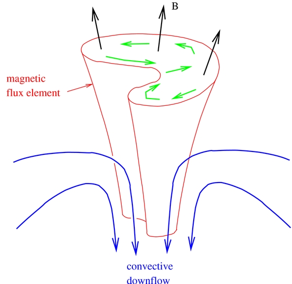
Figure 1. Interaction of a magnetic flux element with convective flows in an intergranular lane. The red object indicates the magnetic element containing a nearly vertical magnetic field, as indicated by the black arrows. The blue arrows indicate the convective flow, which push on the flux tube from one side. Due to the stiffness of the magnetic field, horizontal momentum is transported upward, which results in a distortion of the shape of the flux tube and generates transverse motions inside it (green arrows). We suggest these transverse motions create Alfvén waves that propagate into the upper atmosphere.
Download figure:
Standard image High-resolution imageThe chromosphere is a conduit for the transport of mass and energy into the corona. Actually, only a small fraction of the nonthermal energy injected into the solar atmosphere is transmitted to the corona; most of the energy is dissipated in the lower atmosphere. Therefore, to understand the heating of the Sun's upper atmosphere it is important to study the structure, dynamics, and heating of the chromosphere. High-resolution observations of the chromosphere have shown that it has a complex thermodynamic structure that is strongly influenced by the presence of magnetic fields (see reviews by Judge 2006; Rutten 2007). The chromosphere is highly dynamic and is filled with jet-like features such as mottles and dynamic fibrils on the solar disk (Rouppe van der Voort et al. 2007; De Pontieu et al. 2007a) and spicules at the limb (De Pontieu et al. 2007b). Realistic three-dimensional MHD models of spicule-like structures have been developed (e.g., Martinez-Sykora et al. 2009). Internetwork regions on the quiet Sun are affected by p-mode waves that travel upward from the photosphere and produce shocks that cause intermittent heating (Carlsson & Stein 1997; Ulmschneider et al. 2005). These shocks produce distinct asymmetries in the profiles of the Ca ii H&K lines. However, the magnetic network and plage regions appear to be heated in a different way (Hasan & van Ballegooijen 2008). First, these regions are continually bright in the cores of the Ca ii H&K and Ca ii 8542 Å lines, and the width of the Hα line is enhanced compared to the non-magnetic surroundings (Cauzzi et al. 2009), indicating that the magnetic chromosphere is heated by a sustained heating process. Second, the wavelength profiles of the Ca ii H line from network/plage elements are symmetric with respect to the rest wavelength (e.g., Lites et al. 1993; Sheminova et al. 2005), indicating that the heating is not due to acoustic shock waves. In this paper, we investigate whether the heating of the magnetized chromosphere may be due to dissipation of Alfvén waves as suggested by De Pontieu et al. (2007b).
The paper is organized as follows. In Section 2, the observational constraints on braiding models are discussed. It is shown that, if the corona is heated by dissipation of braided fields, the braiding must occur on small transverse length scales (less than a few arcseconds). This motivates us to develop a three-dimensional MHD model for the dynamics of Alfvén waves inside a magnetic flux tube extending from the photosphere through the chromosphere into the corona. The MHD model is described in Section 3, and modeling results are presented in Section 4. The results are further discussed in Section 5.
2. OBSERVATIONAL CONSTRAINTS ON MAGNETIC BRAIDING MODELS
2.1. Searching for Evidence of Braided Fields
Active regions contain loop-like structures that are aligned with the direction of the coronal magnetic field. In this section we use data from the X-Ray Telescope (XRT; Golub et al. 2007; Kano et al. 2008) on Hinode (Kosugi et al. 2007) to search for braided magnetic fields in the corona. Figure 2(a) shows active region AR 11041 observed on 2010 January 25, starting at 11:02 UT. The observation used the Ti-poly filter, which is sensitive to plasma with temperatures greater than 1 MK. In order to improve the signal-to-noise ratio, we added 12 exposures with exposure time 0.51 s, taken over a period of 50 minutes. Figure 2(b) shows a spatially filtered image where the high spatial frequencies have been enhanced to bring out the loop structures.
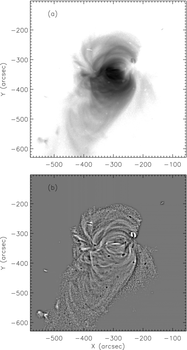
Figure 2. (a) XRT image of active region AR 11041 on 2010 January 25, taken with Ti-poly filter. The image is an average over the period 11:02 UT to 11:52 UT and shows the logarithm of the intensity displayed as a negative (black and white differ by a factor of 100 in intensity). The x and y coordinates are relative to solar disk center. (b) Spatially filtered version of the same image (the dark spots are artifacts due to contamination on the CCD). Note that some of the loops appear to cross each other. The number of loop crossing is much less than one would expect if the corona contained braided magnetic fields on scales ℓ > 5 arcsec.
Download figure:
Standard image High-resolution imageThe structure of the emission is complex, and multiple structures are superposed along the line of sight. There are some distinct coronal loops, but there is also a more diffuse emission component. The loop widths vary from about 3 arcsec for the narrowest loops to about 20 arcsec for the widest ones. The wider loops show some variation in X-ray brightness across the loop on a scale of a few arcseconds, and these fine-scale structures appear to be aligned with the loop axis. However, our ability to observe these features is limited by the spatial resolution of XRT and (for the outer parts of the AR) by photon noise.
The wrapping of bright loops around each other has occasionally been observed with the Transition Region and Coronal Explorer (TRACE; see examples in Schrijver et al. 1999), but these cases are often ambiguous and most loops observed with TRACE do not show evidence for magnetic braiding. To search for braided fields with XRT, we looked for places in Figure 2 where two loops appear to cross each other. There are only a few such sites within the observed active region. If the magnetic field were braided on observable scales (greater than 5 arcsec), one would expect to find many more such loop crossings. The few examples that can be found seem to involve loops that are well separated in height, and do not appear to be due to braided structures. For the wider coronal loops, it appears that the different threads within the loop are co-aligned to within a few degrees, not 20° as predicted by Parker's original braiding model (Parker 1983; Priest et al. 2002; Klimchuk 2006). We conclude there is no evidence for the existence of strongly braided magnetic fields in the corona on spatial scales of a few arcseconds or larger. If there is braiding on the Sun, it must occur on small transverse scales (less than 5 arcsec) and involve small misalignment angles (at most a few degrees).
2.2. The Coronal Heating Rate
An important constraint on any model for coronal heating is that it must explain the average heating rate. The observed radiative and conductive losses of active regions imply a nonradiative energy flux into the corona Fmech ∼ 107 erg cm−2 s−1 (Withbroe & Noyes 1977). Assuming that this energy enters a coronal loop at both ends and is distributed uniformly over the full length Lcor of the loop, the average volumetric heating rate Qcor = 2Fmech/Lcor. For a loop with constant cross section and length Lcor ≈ 50 Mm we obtain Qcor ∼ 4 × 10⁻³ erg cm−3 s−1. Another method for estimating the heating rate is to use the scaling laws first developed by Rosner et al. (1978, hereafter RTV):


where Tmax is the peak temperature (in K), pcor is the coronal plasma pressure (in dyne cm−2), and Lcor is the loop length (in cm or Mm). X-ray observations indicate that the loops in the core of an active region have high temperature and pressure, Tmax ≈ 2.5 MK and pcor ≈ 2 dyne cm−2 (e.g., Saba & Strong 1991; Brosius et al. 1997; Winebarger et al. 2008; Warren et al. 2008; Ugarte-Urra et al. 2009). Assuming a loop length Lcor ≈ 50 Mm, the required heating rate is about 2.9 × 10⁻³ erg cm−3 s−1.
Can the quasi-static braiding models explain such heating rates? In Parker's original model (Parker 1972, 1983) it is assumed that there exist distinct “flux tubes” that can be traced from the corona into the photosphere. These flux tubes are assumed to retain their identity for about 1 day as their footpoints are moved around on the photosphere, and thin current sheets develop at the interfaces between the flux tubes (Berger 1991, 1993; Wilmot-Smith et al. 2009; Berger & Asgari-Targhi 2009). To explain the observed heating rates, large departures from the potential field must develop. Specifically, the angle θ between the braided field B(r) and the potential field B0(r) must be about 20° (Parker 1983; Priest et al. 2002; Klimchuk 2006), otherwise the Poynting flux into the corona is insufficient to balance the observed radiative and conductive losses. These large deviations from the potential field are predicted to occur on transverse scales of a few megameters or larger, and therefore should be readily observable in the fine structures of coronal loops. As discussed in Section 2.1, there is no observational evidence for braided fields on such scales. Therefore, it appears that Parker's original version of the braiding model (with relatively long-lived flux tubes braided on observable scales) is incompatible with coronal observations.
In other braiding models the boundary flows are incompressible and vary randomly with time. This implies that any two points on the boundary tend to separate from each other (e.g., van Ballegooijen 1988), hence there are no well-defined “flux tubes” that retain their identity for many hours. This type of model is consistent with the observation that photospheric flux elements frequently split up and merge (Berger & Title 1996). The magnetic fields produced in such models are more fragmented than those predicted by Parker's original model. Specifically, current sheets can develop anywhere within the volume, and the strongest currents will develop in locations where the footpoint motions have the largest cumulative shear. Analytic studies predict a rapid “cascade” of magnetic energy to small transverse scales (van Ballegooijen 1985, 1986). In fact, the cascade proceeds so rapidly that the energy is dissipated before strong departures from the potential field can develop. As a result, these simple cascade models have difficulty explaining the observed rate of coronal heating in active regions. The model predicts that the coronal heating rate per unit volume is given by

where B0 is the coronal field strength, u0 is the rms velocity of the footpoint motions, τ0 is the correlation time, and Rm is the magnetic Reynolds number (see van Ballegooijen 1986). For motions induced by the solar granulation, τ0 ∼ 5 minutes, which is slow compared to the coronal Alfvén travel time (τ0 ≫ L/vA, where vA is the Alfvén speed, vA ∼ 1000 km s−1). Therefore, the magnetic field is expected to evolve through a series of nearly force-free equilibrium states. Note that Qcor is proportional to the product u20τ0, which is essentially the photospheric diffusion constant, in this model. Therefore, measurements of D can be used as a constraint on the braiding model. Using D ≈ 250 km2 s−1 (DeVore et al. 1985), it was found that the heating rate predicted by the cascade model is a factor of 10 to 40 smaller than the heating rate observed in active regions.

Numerical simulations of magnetic braiding driven by slow, random, incompressible footpoint motions (e.g., Mikić et al. 1989; Longcope & Strauss 1994; Hendrix & van Hoven 1996; Hendrix et al. 1996; Galsgaard & Nordlund 1996; Craig & Sneyd 2005) predict heating rates that are basically consistent with Equation (3). Therefore, like the above cascade model, these numerical models also cannot explain the observed heating rate when realistic values for the random walk diffusion constant D are inserted into the model. We conclude that neither Parker's original version of the braiding model nor its later modifications can adequately explain the structure and heating of coronal loops in active regions. This leads us to consider other types of footpoint motion, such as small-scale random motions inside the photospheric flux elements (see Figure 1).
3. ALFVÉN WAVE TURBULENCE MODEL
A model for the dynamics of plasma and magnetic field inside a coronal loop is developed. We consider only a thin tube of magnetic flux, corresponding to a single kilogauss flux tube in the photosphere. The tube extends from the photosphere at one end of the loop, through the chromosphere into the corona, and back down into the photosphere at the other end. In the photosphere and chromosphere the flux tube is assumed to be vertically oriented. We assume that a single flux tube at one end of the loop is connected to a single flux tube at the other end, i.e., we ignore the fact that on the real Sun the photospheric flux concentrations at the two ends are uncorrelated and do not perfectly match up. Also, on the real Sun magnetic flux elements frequently split up and merge with their neighbors (Berger et al. 1995; Berger & Title 1996; van Ballegooijen et al. 1998). Such processes may lead to magnetic reconnection and may be important for coronal heating (e.g., Furusawa & Sakai 2000; Sakai & Furusawa 2002). However, in the present model we neglect such effects, and we assume that the flux tube retains its identity for the duration of the simulation.
The tube has a length L, and the overall curvature of the tube is neglected. We use a coordinate system (x, y, z), where z is the coordinate along the tube axis (0 ⩽ z ⩽ L), and x and y are perpendicular to the axis. Note that near the “left” end of the flux tube (z ≈ 0) the height in the lower atmosphere is given by z and gravity acts in the direction, but near the “right” end (z ≈ L) the height is given by L − z and gravity is in the direction. Despite these differences, we will sometimes refer to z simply as the “height” in the flux tube. The tube is assumed to have a circular cross section with radius R(z), which is much smaller than its length L. To simulate the effects of solar convection interacting with the flux tube, we impose random footpoint motions on the field lines at the base of the photosphere (z = 0 and z = L). These motions produce Alfvén waves that travel along the flux tube, reflect due to gradients in Alfvén speed, and generate turbulence via nonlinear wave–wave interactions. The dynamics of the waves inside the tube are described by the equation of motion,


and the magnetic induction equation,

Here ρ(r, t) is the plasma density, p(r, t) is the pressure, v(r, t) is the velocity, B(r, t) is the magnetic field, is the acceleration of gravity, and Dv and Dm are viscous and resistive dissipation terms. The magnetic field satisfies the solenoidal condition, ∇ · B = 0. The velocity v can be split into parallel and perpendicular components:


where is the unit vector along the perturbed magnetic field and . Taking the inner product of Equation (4) with , we obtain


The first term on the right-hand side is the centrifugal force due to changes in the shapes of the magnetic field lines, which is an important driver of field-aligned flows. However, in the present paper we will neglect parallel flows and focus on the perpendicular motions of the plasma. Note that, according to Equation (5), the parallel velocity v∥ has no direct effect on the evolution of the magnetic field.
In this paper, we use the so-called reduced MHD (RMHD) approximation (Strauss 1976), which assumes that the magnetic fluctuations are small compared to the background field. In subsection 3.1, we present a derivation of the RMHD equations in the context of the present model. In the following subsections we describe the structure of the background atmosphere, the imposed footpoint motions, and the numerical techniques for solving the RMHD equations. Subsection 3.5 describes some of the limitations of the present model.
3.1. Reduced MHD Equations for a Nonuniform Medium With Gravity
In this section, we derive the RMHD equations describing the nonlinear dynamics of Alfvén waves in a flux tube with non-constant cross section and with density varying by orders of magnitude along the flux tube. The RMHD equations were first derived by Kadomtsev & Pogutse (1974) and Strauss (1976) for a uniform background field (also see Montgomery 1982; Hazeltine 1983), and the relationships between compressible MHD, incompressible MHD, and RMHD were extensively discussed by Zank & Matthaeus (1992). Schekochihin et al. (2009) considered the extension of the RMHD equations into the kinetic regime. Bhattacharjee et al. (1998) included the effects of plasma pressure, spatial inhomogeneities, and parallel flows into the formalism, and they derived a more general set of four coupled equations. However, they did not include the effects of gravity. In the absence of gravity, the magneto-static equilibrium equation implies that the gradient of the plasma pressure is perpendicular to the mean magnetic field, ∇p0⊥B0. In contrast, in the present case gravity plays an important role in the stratification of the plasma pressure p0(z) and density ρ0(z) in the photosphere and chromosphere, and at the axis of the flux tube ∇p0∥B0. Therefore, the four-field equations derived by Bhattacharjee et al. (1998) cannot be directly applied to the present case. Also, many analyses of the RMHD equations use normalized dynamical variables, which makes sense when the background density is roughly constant, but not when ρ0 varies by several orders of magnitude within the system. This makes it necessary to discuss in some detail the assumptions underlying the equations used in the present work.
Our starting point is the equation of motion (4). The magnetic and velocity fields are written as sums over mean and fluctuating components, B = B0 + B1 + ⋅⋅⋅ and v⊥ = v⊥, 0 + v⊥, 1 + ⋅⋅⋅, and similar for the parallel velocity, density, and pressure. The background field B0 is nonuniform and varies on a spatial scale HB, which is defined by

where B0(r) is the background field strength and is the unit vector along the background field. We assume that the background atmosphere is in static equilibrium (v⊥, 0 = 0 and v∥, 0 = 0), and that the interior of the flux tube is current free, ∇ × B0 = 0, i.e., all currents are located at the interface between the flux tube and its surroundings. Then Equation (4) yields ∇p0 = ρ0g, where p0(z) and ρ0(z) are the unperturbed pressure and density as functions of height z inside the flux tube.

We now assume that the radius R(z) of the flux tube is small compared to the length scale |HB(z)| of the magnetic field inside the tube. Then we can define a small parameter,

and the background field B0(r) can be approximated as

where B00(z) is the field strength on the tube axis (x = y = 0). The unit vector along the background field is given by

where we used HB(z) ≈ B00/(dB00/dz). Flux conservation implies that B00R2 ≈ constant along the flux tube. Note that ∇ · B0 = 0 as required, and that the unit vector varies over the cross section of the flux tube:

The above “thin tube approximation” has been used by many authors to study waves and instabilities in flux tubes (e.g., Defouw 1976; Roberts & Webb 1978; Spruit 1981).
We now consider the perturbations due to Alfvén waves that are launched at the base of the photosphere (z = 0 and z = L) and are reflected in the chromosphere and at the TR. The velocity amplitude u⊥(z) of the waves is assumed to be small compared to the Alfvén speed vA(z), so that the magnetic perturbation B1(r, t) is small compared to the background field B00(z). Furthermore, we assume that the transverse length scale ℓ⊥ of the waves is less than the tube radius (ℓ⊥ ⩽ R) and is small compared to the parallel scale ℓ∥. The latter is defined by

where τ is the typical timescale of the magnetic fluctuations (e.g., the Alfvén wave period), |HB| is the length scale of the background field, and L is the loop length. Then we can define a second small parameter:

and we can expand the magnetic and velocity fields in powers of  :
:


where in general , and . We assume that the main driver of parallel flows is the centrifugal force given by the first term in Equation (7). Then the parallel velocity .


In some derivations of the RMHD equations (e.g., Strauss 1976; Montgomery 1982) it is assumed that the plasma flow is incompressible, ∇ · v ≈ 0, but others have argued that this assumption cannot be taken for granted when the plasma beta is of order unity (e.g., Zank & Matthaeus 1992). Here β ≡ 8πp0/B20 is the ratio of gas pressure and magnetic pressure. For the models presented in this paper, β ∼ 1 in the photospheric part of the flux tube (see Section 3.2). It is not clear from the literature on the RMHD equations whether the assumption of incompressibility is still valid when β ∼ 1 and the background medium is nonuniform. Therefore, we must first estimate the magnitude of ∇ · v for our particular model and determine whether the assumption of incompressibility is still valid. Using Equation (6), the velocity divergence can be written as

The second term is of the order of vA3/ℓ⊥, but the magnitude of the first term is unclear. To estimate this term, we insert expressions (15) and (16) into the momentum Equation (4), omitting the dissipative term, and then take the divergence, which yields

It follows that the perturbation of the total pressure is of second order in (Zank & Matthaeus 1992; Bhattacharjee et al. 1998):

Also, taking the inner product of Equation (5) with B/4π, we obtain

where we used Equation (4), again without the dissipative term. Inserting expressions (15), (16), and (19), we find

Finally, the pressure is assumed to evolve adiabatically, dp/dt = −γp∇ · v, where γ is the ratio of specific heats. In lowest order of this equation becomes

where we used v · ∇p0 ∼ vA2|dp0/dz|. Adding Equations (21) and (22), and dividing by the factor (γp0 + B20/4π), we find

i.e., the magnitude of ∇ · v⊥ is of third order in . Inserting this result into Equation (22), we find , so the pressure variations are really of second order in , and we can set p1 = 0. Inserting p1 = 0 into Equation (19), we find , so the first-order perturbation of the magnetic field is perpendicular to the background field, B1⊥B0. Therefore, the effects of compressibility can be neglected in the present models, ∇ · v⊥ = 0, even though β ∼ 1 in some regions of the model. This is due to the fact that the transverse motions of the waves are nearly horizontal and therefore along the planes of constant pressure p0(z) inside the flux tube.


The induction equation (5) can also be written as

where A(r, t) is the vector potential (B ≡ ∇ × A), ϕ(r, t) is the electric potential, and we omit the dissipative term. From the above analysis it is clear that the Lorentz force is of order 2, so the component of electric current perpendicular to B0 is also of this order (Strauss 1997). Therefore, the first-order perturbation of the vector potential must be parallel to the background field:

where h is the magnetic flux function (h ∼ ℓ⊥). Using ∇ × B0 = 0, we find B1 = ∇h × B0, which is perpendicular to B0 as required. Then the total magnetic field is

Here ∇⊥ is defined in relation to the background field, , whereas v⊥ is defined to be perpendicular to the perturbed field B. Inserting expression (25) into (24) and taking the inner product with B, we obtain


where we use B · B0 = B20. Taking the cross product of Equation (24) with B0 and using the condition v⊥ · B = 0, we find

where ξ ≡ −∇⊥ϕ · ∇⊥h. The two terms with ϕ and ξ are of order vA and vA2, respectively. Taking the divergence of Equation (28), we obtain

Estimating the magnitudes of the various terms and using the fact that ∇B0 is nearly parallel to B0, we find that all terms are of the order of vA3/ℓ⊥, so Equation (29) is consistent with Equation (23). Neglecting terms of order 2 in Equation (28), the perpendicular velocity can be further approximated as

where f ≡ ϕ(r, t)/B0(r). In this approximation the component of v⊥ parallel to B0 is neglected. The quantity f(r, t) can be interpreted as the velocity stream function. Inserting the expression ϕ = fB0 into Equation (27), we obtain for the magnetic induction equation:

We now consider the equation of motion (4). As discussed above, we can neglect the fluctuations in gas pressure and density (p1 = ρ1 = 0), and we also omit the viscous term. Using Equations (12) and (26), the curl of the magnetic field can be approximated as

where α is defined by

Inserting expression (32) into Equation (4), we find for the acceleration perpendicular to B0:

where . We now consider the parallel component of the vorticity equation. Using Equation (30), the parallel vorticity can be approximated as


and using , the inertial term in Equation (34) becomes


The cross-product on the right-hand side of Equation (34) yields

where Equation (12) is used several times, and HB eventually drops out of the expression. Therefore, we obtain the following scalar form of the vorticity equation:

Here vA depends on position z along the flux tube and depends on x and y as described by Equation (12). The magnetic field strength B0 is nearly constant over the cross section of the tube and can be approximated by its value on axis, B0 ≈ B00(z). Therefore, in the remainder of this paper we will write the magnetic field strength as B0(z).

The last step is to replace ∇⊥ with in the definitions of α and ω, and in the nonlinear terms of Equations (31) and (38), but not in the linear terms where quantities are differentiated along the background field. Then ∇2⊥ ≈ ∂2/∂x2 + ∂2/∂y2, and the dynamical Equations (31) and (38) can be written as


where [⋅⋅⋅, ⋅⋅⋅] is the bracket operator:

We also derive an alternative form of the dynamical equations. Taking the second derivative of Equation (39), we find

where we used Equation (12) to evaluate the horizontal derivatives of (note that HB is eliminated from the equation). In analogy with the Elsasser variables (Elsasser 1950), we define


and inverting these relations, we can write f = (f+ + f−)/2, h = (f+ − f−)/(2vA), ω = (ω+ + ω−)/2, and α = (ω+ − ω−)/(2vA). Therefore, combining Equations (40) and (42), we obtain the following equations for ω±:

where the nonlinear term is defined by


The equations for ω+ and ω− describe inward and outward propagating Alfvén waves, respectively ( directions); the term with dvA/dz describes linear coupling between these waves; and the last two terms describe nonlinear coupling. In Appendix A we demonstrate that Equation (44) is consistent with earlier formulations of the wave transport equations based on the Elsasser variables. The numerical methods used in solving these equations are discussion in Section 3.4 and Appendix B.

3.2. Background Atmosphere
We now describe the undisturbed state of the flux tube before any waves are injected. In the closed field case there are two “lower atmospheres” located at each end of the flux tube. The chromosphere–corona TRs are located at positions z = zTR and z = Lcor + zTR, where zTR is the height of the first TR, and Lcor is the coronal loop length. The total length of the tube is L = Lcor + 2zTR. The gas pressure p0(z), density ρ0(z), and magnetic field strength B0(z) are functions of z only, i.e., we neglect variations of these quantities in planes perpendicular to the flux tube axis. Furthermore, the functions p0(z), ρ0(z), R(z), and B0(z) are assumed to be symmetric with respect to the mid-point of the loop (z = L/2), so the two halves of the loop are identical.
The structure of the lower atmosphere is based on a model of a facular region (i.e., very bright plage region) called model P, which was first developed by Fontenla et al. (1999) and more recently discussed by Fontenla et al. (2006, 2009). The temperature T0(z) and molecular weight μ0(z) are specified as a function of height to be in rough agreement with this model. At the base of the photosphere, we assume B0(0) = Bphot = 1400 G and p0(0) = 3 × 10⁴ dyne cm−2, which is the internal pressure of the flux tube; then the total pressure (p0 + B20/8π) is about 1.1 × 10⁵ dyne cm−2, consistent with model P. The gas pressure p0(z) and density ρ0(z) as functions of height are determined by solving a modified hydrostatic equilibrium equation, dp0/dz = −ρ0geff, where geff is the gravitational acceleration corrected for the effects of turbulent motions. The pressure at the TR is given by

where zTR is in Mm. The magnetic field strength in the lower atmosphere is given by

where Bphot = 1400 G and Bcor is the field strength at the coronal base (i.e., at z = zTR). In the photosphere p0 ≫ p0(zTR) and B0 ≫ Bcor, so that the ratio of gas and magnetic pressures is approximately constant:

At larger heights in the chromosphere B0(z) approaches the coronal value and β(z) decreases with height to values well below unity.
In the TR the temperature T0(z) increases rapidly with height from about 104 K in the upper chromosphere to about 106 K in the corona. We do not attempt to resolve this temperature structure, and treat it as a discontinuity. For closed loops we use the following profile for the temperature in the corona:

where u(z) ≡ −1 + 2(z − zTR)/Lcor, which lies in the range −1 ⩽ u ⩽ +1, and Tmax is the peak temperature in the loop as predicted by the RTV scaling law, Equation (1). It follows that T0(zTR) = 0.631Tmax, so the temperature in the upper TR is a fixed fraction of the peak temperature in the corona. The above profile is similar to that predicted for a conduction-dominated loop with constant cross section and uniform heating (e.g., Vesecky et al. 1979; Martens et al. 2000; Martens 2010). Although it is not difficult to include the effects of gravity (e.g., Serio et al. 1981), in this paper we neglect gravity in the corona, so that the gas pressure p0(z) is constant along the coronal part of the loop. The pressure is continuous across the TR, so the coronal pressure pcor = p0(zTR). Therefore, the coronal pressure is determined by the height zTR of the TR. The plasma density in the corona is given by

where ρ0(zTR) is the density at the coronal base, which is computed from pcor and T0(zTR). For closed loops the coronal field is approximated as

where Γ is the areal expansion factor; for open fields we use B0(z) = Bcor = constant in the corona. In either case the magnetic flux Φ (=πR2B0) is constant along the flux tube, so the tube radius is given by

Here, Rphot = 100 km is the tube radius at the base of the photosphere (z = 0 and z = L). The radius R in the corona depends on the parameters Bcor and Γ and is different for the different models.
We consider a reference model with coronal field strength Bcor = 50 G, expansion factor Γ = 1, and TR height zTR = 1.8 Mm, which corresponds to a coronal pressure pcor = 1.833 dyne cm−2. The coronal loop length Lcor = 49.6 Mm, which is the closest one can get to 50 Mm with the chosen time step Δt0 = 0.746 s (see Appendix B for details). The total loop length is L = 53.6 Mm. Figure 3 shows various quantities plotted as a function of position along the flux tube for this model. Positions are given in terms of the Alfvén wave travel time from the left footpoint (z = 0):

Figure 3(a) shows the relationship between z and τ for the reference model; the photospheric footpoints are located at τ(0) = 0 and τ(L) = 190.9 s, and the corona is located in the region 81.3 s < τ < 109.6 s. The other panels in Figure 3 show the temperature T0, density ρ0, magnetic field strength B0, flux tube radius R, the absolute value of the magnetic scale height HB (defined in Equation (8)), and the Alfvén speed vA as functions of Alfvén travel time τ from the left footpoint. Note that when expressed in terms of τ, the corona is only a small part of the computational domain.
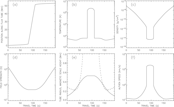
Figure 3. Reference model for a coronal loop and the two “lower atmospheres” at the two ends of the loop. Various quantities are plotted as a function of the Alfvén wave travel τ to a given point along the loop: (a) position z(τ) along the loop as measured from the left footpoint, (b) temperature T0, (c) mass density ρ0, (d) magnetic field strength B0, (e) flux tube radius R (full curve) and magnetic scale height |HB| (dashed curve), and (f) Alfvén speed vA. The two chromosphere–corona TRs are located at τ = 81.3 s and τ = 109.6 s.
Download figure:
Standard image High-resolution imageFigure 3(e) shows that |HB| < R in two intervals, 30 s < τ < 48 s and 140 s < τ < 158 s, which correspond to the temperature minimum regions at the two ends of the loop. In these regions the quantity 0 defined in Equation (9) is greater than unity, so the thin tube approximation is no longer valid. Clearly, the thin tube and RMHD approximations discussed in Section 3.1 provide only a crude description of the magnetic structure and wave dynamics in the lower atmosphere. A proper treatment will require full MHD simulations and is beyond the scope of the present work.
The present model predicts braiding of the coronal field lines on a transverse scale less than the tube radius, Rcor ≈ 529 km. This radius is less than the resolution limits of present-day XRTs. Therefore, we should expect that the predicted coronal structures will be difficult to observe.
3.3. Photospheric Footpoint Motions
The Alfvén waves are produced by footpoint motions imposed at the two ends of the flux tube, z = 0 and z = L. In reality these motions may distort the shape of the flux tube as indicated in Figure 1, but here we use a simpler approach in which the motions are assumed to be confined to a circular area x2 + y2 ⩽ R2phot at z = 0 and similar at z = L. The velocity v(x, y, 0, t) at these boundaries can be written in terms of polar coordinates (r, φ), where r is the distance from the flux tube axis and φ is the azimuth angle in the (x, y) plane. We assume that the radial component of velocity vanishes at the tube wall, vr(Rphot, φ, 0, t) = 0, so that the circular shape of the cross section is preserved. We also assume that the motions are horizontal and incompressible:

where f(r, φ, 0, t) is the stream function at z = 0 and similar at z = L. As described in Appendix B, functions on a circular area can be decomposed into orthogonal basis functions Fi(ξ, φ), where ξ is the relative distance from the tube axis (ξ ≡ r/R) and index i enumerates the basis functions (i = 1, …, N). We use a relatively small number of basis functions (N = 92); the functions are shown in Figure 13.
In this paper we assume that the footpoint motions have a pattern consisting of two counter-rotating cells. This pattern can be described as a superposition of two modes with azimuthal mode number m = 1. For the particular set of basis functions used in the present paper, these driver modes have indices i = 7 and i = 8 (see Appendix B for details), and are shown in the top row of Figure 13 (seventh and eighth image from the left). Both modes have the same radial dependence given by J0(a⊥r/Rphot), where J0(x) is the zeroth-order Bessel function of the first kind and a⊥ is the dimensionless perpendicular wavenumber, which equals 3.832 for these particular modes (the first zero of the Bessel function). However, the azimuth dependence of the two modes is different: the mode with i = 7 is proportional to cos φ, while the one with i = 8 is proportional to sin φ. The imposed stream function at z = 0 can then be written as a superposition of the two modes:

Here, f7(t) and f8(t) are the mode amplitudes, which vary randomly with time t and are not correlated with each other. The vertical component of vorticity at z = 0 is then given by

The above time-dependent pattern simulates the intermixing of the plasma within the flux tube due to motions imposed by the surrounding convective flows.
The random variables f7(t) and f8(t) are constructed as follows. For each variable, we first create a normally distributed random sequence f(t) on a grid of times covering the entire length of the simulation (tmax = 3000 s). Then the sequence is filtered in the Fourier domain using a Gaussian function, , where is the temporal frequency (in Hz) and τ0 is the specified correlation time (for the reference model τ0 = 60 s). The filtered sequence is renormalized such that the rms vorticity of each mode equals a specified value, ω0. The rms velocity of the combined pattern of the two modes is . The quantities τ0 and ω0 are free parameters of the model.
![$G(\tilde{\nu }) = \exp [-(\tau _0 \tilde{\nu })^2]$](https://content.cld.iop.org/journals/0004-637X/736/1/3/revision1/apj392169ieqn25.gif)


3.4. Numerical Methods
The techniques used for solving the RMHD equations are described in Appendix B and the energy equation is discussed in Appendix C. The transverse dependence of the waves is described using a spectral method, i.e., all scalar functions are written as sums over 92 discrete modes. The nonlinear terms in the equations are represented by a matrix Mkji that couples the different modes and cause transfer of energy from low to high wavenumber. The modes with the highest transverse wavenumbers are artificially damped, which describes viscous and resistive processes on small spatial scales. The damping rate is given by Equation (B13) with νmax = 0.7 s−1. For the z dependence of the waves we use finite differences, for example, in the model shown in Figure 3 there are 259 points along the tube. To accurately simulate the wave propagation, we use a grid that is uniform in Alfvén wave travel time τ(z) with a grid spacing Δτ equal to the time step Δt0 of the simulation (for the reference model, Δt0 = 0.746 s). At the chromosphere–corona TR the density ρ0(z) is discontinuous, which is represented by two grid points at the same position zTR but with different densities. The discontinuity causes wave reflections that are described in terms of reflection and transmission coefficients (see Appendix B for details).
The RMHD model is valid only when ΔBrms/B0 ≪ 1, where ΔBrms is the rms value of the transverse magnetic field fluctuation. We will find that this condition is only marginally satisfied. Therefore, the present model can describe only some of the dynamical processes that occur in the chromosphere and corona. In particular, the model does not describe field-aligned flows such as spicules.
3.5. Limitations of the Model
The present model for chromospheric and coronal heating has several drawbacks and limitations. The code uses an explicit numerical scheme, which makes it difficult to simulate waves in models with high coronal field strength. On the real Sun the field strength in active region loops in the low corona is 100–500 G, but in the present paper we must limit ourselves to Bcor ⩽ 200 G. Also, the model includes only a limited number of wave modes (see Figure 13), and the time step is relatively large (Δt0 > 0.1 s), so the turbulent spectrum is not well resolved.
The model considers only a single magnetic flux tube, and does not allow for splitting and merging of magnetic flux elements at the two ends of the coronal loop (Berger & Title 1996). It is unclear to what extent the chromospheric and coronal heating rates and the spatial distribution of the heating are affected by this approximation. Perhaps more importantly, the present RMHD model does not allow for feedback of the heating on the background atmosphere. In the present version there are no field-aligned flows, and the temperature and density are assumed to be constant in time, so we do not simulate the dynamic response of the atmosphere to heating events. This also means that we cannot make predictions regarding the temporal variability of EUV and X-ray emissions from the modeled coronal loops. In particular, we do not simulate spicules or similar dynamic events, even though such events may in fact be driven by nonlinear Alfvén waves (see Matsumoto & Shibata 2010). The plasma density in our model is assumed to be constant in planes perpendicular to the tube axis, so there are no variations in density on scales less than the tube radius. Therefore, the present model has little to say about the multi-thermal structure of coronal loops.
Finally, the model does not include the effects of phase mixing (Heyvaerts & Priest 1983) or resonant absorption (e.g., De Groof & Goossens 2002), which depend on the variation of Alfvén speed in the plane perpendicular to the tube axis. In the present model both B0 and ρ0 are constant in the (x, y) plane.
4. RESULTS
4.1. Reference Model
We first construct a reference model with coronal field strength Bcor = 50 G, expansion factor Γ = 1, and coronal loop length of about 50 Mm. More precisely, the coronal loop length Lcor = 49.6 Mm, the transition-region height zTR = 1.8 Mm, and the total tube length L = 53.2 Mm. The footpoint motions have a correlation time τ0 = 60 s, each of the driver modes has a vorticity ω0 = 0.04 s−1, and the rms velocity is Δvrms = 1.48 km s−1. The latter is reasonable compared to the convective velocities of several km s−1 expected to exist in the downflow lanes below the photosphere. The TR height corresponds to a coronal pressure pcor = 1.833 dyne cm−2, which is typical for hot loops found in active regions, and Equation (1) yields a peak temperature Tmax = 2.3 MK.
The vorticities of the driver modes are shown as a function of time in Figures 4(a) and (b) for the left (z = 0) and right (z = L) footpoints, respectively. These random footpoint motions create Alfvén waves that propagate upward along the flux tube. Initially, only the two driver modes are present. The decrease of density with height causes the velocity amplitude of the waves to increase with height. In the chromosphere, part of the wave energy is reflected back down due to the increase of Alfvén speed with height. Even stronger reflection occurs at the chromosphere–corona TR, where the Alfvén speed suddenly increases by about a factor of 15. These reflections produce a pattern of counter-propagating waves in the photosphere and chromosphere at the two ends of the loop. The wave amplitudes in the chromosphere soon build up to about 20–30 km s−1, consistent with the observations by De Pontieu et al. (2007b).
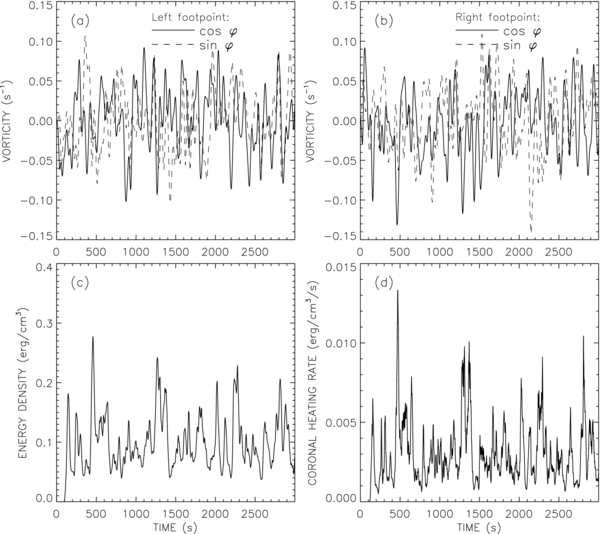
Figure 4. Various quantities plotted as a function of time for the reference model: (a) imposed vorticity ωk at the left footpoint (z = 0) for k = 7 (full curve) and k = 8 (dashed curve); (b) similar for the right footpoint (z = L); (c) energy density E in the corona; and (d) coronal heating rate, Qcor.
Download figure:
Standard image High-resolution imageDue to evolution of the driver modes and time delays in the reflection, the inward and outward propagating waves at a given height z have different spatial distributions in the (x, y) plane. Furthermore, these patterns are superpositions of multiple modes with different perpendicular wavenumbers. Such counter-propagating waves with different spatial patterns and multiple modes are subject to strong nonlinear interactions (e.g., Shebalin et al. 1983; Higdon 1984; Oughton & Matthaeus 1995; Goldreich & Sridhar 1995, 1997; Bhattacharjee & Ng 2001; Cho et al. 2002; Oughton et al. 2004). In our RMHD model, these interactions are due to the bracket terms in Equations (39), (40), and (44). Basically, the inward propagating waves are distorted by the outward propagating waves, and vice versa (e.g., Chandran et al. 2009). These distortions are large because the fluid displacements are comparable to the transverse scale of the waves. For example, for chromospheric waves with velocity amplitude of 10 km s−1 acting over a period of 50 s, the transverse displacement is about 500 km, equal to the transverse scale of the driver modes. As a result of these nonlinear interactions, other wave modes with smaller spatial scales are excited (see Figure 13 for a display of the 92 wave modes used in the present model). After about 200 s from the start of the simulation, a well-developed spectrum of Alfvén waves has formed and dissipation of the high-wavenumber waves becomes significant. This dissipation is due to a combination of viscous and resistive diffusion effects, so the model includes the effects of magnetic reconnection. Such turbulent dissipation of waves in the lower atmosphere continues throughout the simulation.
A small fraction of the wave energy is transmitted through the TR into the corona. Energy is injected into the coronal loop at both ends, producing counter-propagating waves in the corona. As in the chromosphere, the counter-propagating waves significantly distort each other because (1) they have different spatial patterns and (2) the fluid displacements are comparable to the transverse scale of the waves. Therefore, the waves produce turbulence in the corona, and there is a continual cascade of energy to smaller transverse scales. As a result, part of the Alfvén wave energy is dissipated in the coronal part of the loop, again due to combination of viscous and resistive effects. We find that the rms velocity amplitude of the waves in the corona is similar to that in the upper chromosphere, but the energy dissipation rate in the corona is much lower because of the lower coronal density.
In the present model, all of the dissipation occurs via Alfvén wave turbulence, both in the chromosphere and in the corona. Phase mixing and resonant absorption of Alfvén waves (e.g., Heyvaerts & Priest 1983; Poedts et al. 1989; Ofman et al. 1994; Erdélyi & Goossens 1995; De Groof & Goossens 2002) play no role because these processes require variations in Alfvén speed across the field lines, which are not included in the present model. A key feature of the model is that the photospheric footpoint motions include more than one driver mode, not just the torsional mode as in the simulations by Antolin & Shibata (2010) and Matsumoto & Shibata (2010). Specifically, we use two driver modes (modes k = 7 and k = 8 in Figure 13) with azimuthal mode number m = 1. If the system is driven using only a single mode (e.g., k = 7), all nonlinear terms in Equations (39) and (40) vanish. In this case all energy remains in the driver mode, and no turbulence develops, as we have verified in test calculations. Hence, for Alfvén wave turbulence to develop it is essential that the footpoint motions include multiple driver modes that have nonlinear couplings with high wavenumber modes. This coupling can be indirect; for the chosen m = 1 modes, the coupling runs via the m = 0 modes.
Figure 4(c) shows the spatially averaged energy density of the waves E(t) in the corona as a function of time (average between z = zTR and z = zTR + Lcor). This quantity is the sum of magnetic free energy Emag(t) and kinetic energy Ekin(t), but the magnetic energy dominates. Figure 4(d) shows the spatially averaged heating rate Qcor(t) per unit volume in the corona. Note that both the energy density and the heating rate vary strongly with time. Significant heating starts only after about 200 s when the waves have become sufficiently turbulent. During the latter part of the simulation, the average heating rate in the coronal part of the loop is 2.98 × 10⁻³ erg cm−3 s−1. This is consistent with the second RTV scaling law, Equation (2), which yields Qcor = 2.9 × 10⁻³ erg cm−3 s−1. Therefore, the reference model describes a coronal loop in which the average rate of plasma heating is balanced by radiative and conductive losses. The model represents the kind of hot, dense loops typically found in active regions. We conclude that such loops can be heated by Alfvén wave turbulence generated inside the magnetic flux tubes by footpoint motions with rms velocity of about 1.5 km s−1.
Figure 5 shows various quantities as a function of position along the flux tube, averaged over the cross section of the flux tube (x and y) and over the time interval t = [800, 3000] s. Positions are given in terms of the Alfvén travel time τ(z) in seconds. Figure 5(a) shows the kinetic and magnetic energy densities, Ekin(z) and Emag(z), and their sum E(z). Figure 5(d) shows similar plots for the kinetic and magnetic heating rates, Qkin(z) and Qmag(z), and their sum Q(z). These quantities are discontinuous at the TR. In the deep photosphere (τ < 20 s and τ > 170 s) and in the corona (81.3 s < τ < 109.6 s) the magnetic energy dominates, but in the chromosphere Ekin > Emag; this is similar to what happens in open-field models with non-WKB wave reflection dominated by low-frequency waves (see Figure 6 in Cranmer & van Ballegooijen 2005). Despite these differences in wave energy density, magnetic heating dominates over viscous heating almost everywhere in the model (Qmag > Qkin).
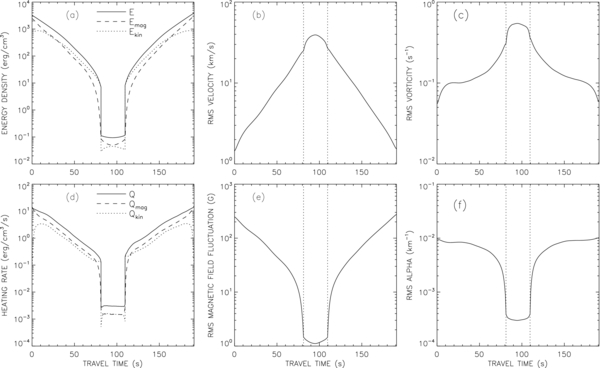
Figure 5. Model for Alfvén wave turbulence in a coronal loop. Various quantities are plotted as a function of position along the flux tube for the reference model: (a) kinetic and magnetic energy densities, and their sum E(z); (b) rms velocity Δvrms; (c) rms vorticity ωrms; (d) kinetic and magnetic heating rates, and their sum Q(z); (e) rms magnetic fluctuation ΔBrms; and (f) rms twist parameter αrms. These quantities are averaged over the cross section of the flux tube and over time. Positions along the loop are given in terms of the Alfvén travel time τ(z). The corona is located in the range 81.3 s < τ < 109.6 s, which is indicated by vertical dotted lines.
Download figure:
Standard image High-resolution imageThe middle and right panels in Figure 5 show the rms values of the velocity, vorticity, magnetic field fluctuation, and α parameter. All four of these quantities are continuous at the TR. The rms velocity Δvrms and rms magnetic field fluctuation ΔBrms are defined in Equations (C1) and (C2), and are further averaged over time. Note that the velocity and vorticity have their peak values at the mid-point of the loop in the corona, Δvrms ≈ 37 km s−1 and ωrms ≈ 0.52 s−1 at τ = 95.4 s (see Figures 5(b) and (c)). Also note that the velocity at the mid-point is about 60% larger than that at the two TRs (vertical dashed lines in 5b). This is due to the fact that the waves in the corona are reflected back and forth between the TRs several times before they decay, creating standing waves with nodes near the TRs. The velocities of 20–40 km s−1 found here for the corona are similar to the nonthermal velocities of 20–60 km s−1 found in observations of spectral line widths in active regions (e.g., Dere & Mason 1993; Warren et al. 2008; Li & Ding 2009) and on the quiet Sun (Chae et al. 1998; McIntosh et al. 2008). This suggests that the modeled waves have more or less the correct amplitude. The magnetic fluctuation ΔBrms(z) and twist parameter αrms(z) shown in Figures 5(e) and (f) have their peaks in the lower atmosphere. This is due to the large gradients in Alfvén speed in the chromosphere and TR, which cause strong wave reflection and produce a patterns of nearly standing waves in the lower atmosphere. The non-constancy of αrms(z) implies that the system is far from a force-free equilibrium state. The peak value of ΔBrms/B0 occurs in the low chromosphere and is about 0.3, so the RMHD approximation is only marginally satisfied.
Figure 6 shows cross sections of the tube at various positions along the loop at the end of the simulation (t = 3000 s). The top row shows the velocity stream function f(x, y, z), the second row shows the vorticity ω(x, y, z), the third row shows the magnetic flux function h(x, y, z), and the bottom row shows the twist parameter α(x, y, z). The different columns corresponds to different positions z along the loop and are labeled with the Alfvén travel time τ(z) from the left footpoint. The two TRs are located at τ = 81.3 s and τ = 109.6 s. The upper left and upper right panels show the footpoint motions that drive the system. The vorticity ω(x, y, z) and twist α(x, y, z) exhibit small-scale structures that are produced by nonlinear interactions, as described above. A movie sequence of such images is available in the online version of the manuscript. This sequence covers the last 298 s of the simulation and shows that the system is highly turbulent. The waves in the corona have smaller spatial scales and evolve more rapidly than those in the lower atmosphere.
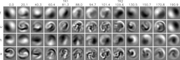
Figure 6. Spatial distribution of various dynamical quantities in the reference model at time t = 3000 s: velocity stream function f, vorticity ω, magnetic flux function h, and twist parameter α. The different columns correspond to different positions along the flux tube and are labeled with the Alfvén travel time τ(z). Each panel shows the normalized distribution of the relevant quantity as a function of transverse coordinates x and y (see Figure 5 for information about the normalization).(An animation of this figure is available in the online journal.)
Download figure:
Standard image High-resolution imageFigures 7(a) and (b) show magnetic field lines in the reference model at time t = 2702 s in the lower atmosphere and in the corona, respectively (the vertical scales of these images are compressed by different factors). The field lines are traced from randomly selected points at height z = 0 in the photosphere. The field lines are significantly distorted due to the Alfvén waves that travel up and down the flux tube with a range of transverse wavenumbers. Two movie sequences of such images are available in the online version of the manuscript. These movies show the evolution of the magnetic field over a period of 298 s (from t = 2702 s to t = 3000 s), and are traced from footpoints that move with the flow. The coronal field lines are to some degree twisted and braided around each other (see Figure 7(b)), but these structures are highly dynamic and change on a timescale of seconds. Therefore, the system is not in a force-free state and is best described as Alfvén wave turbulence. The effects of such turbulence on the solar corona have been modeled previously for both open (Hollweg 1986; Zhou & Matthaeus 1990; Matthaeus et al. 1999; Dmitruk et al. 2001; Dmitruk & Matthaeus 2003; Cranmer & van Ballegooijen 2003, 2005; Cranmer et al. 2007; Verdini & Velli 2007) and closed magnetic fields (Heyvaerts & Priest 1984, 1992; Longcope & Strauss 1994; Dmitruk & Gomez 1997; Buchlin & Velli 2007; Rappazzo et al. 2008). The present work demonstrates that Alfvén wave turbulence can occur both in the chromosphere and in the corona, and can develop even when the photospheric footpoint motions occur on very small spatial scales (ℓ⊥ < 100 km). The model can quantitatively explain the observed heating rates in active regions.

Figure 7. Magnetic field lines in the reference model at time t = 2701.7 s, viewed from an angle of 30°. (a) The lower atmosphere up to the height of the first TR, zTR = 1.8 Mm. The starting points of the field lines are randomly distributed inside the flux tube at height z = 0 (cylinder base). The radius of cylinder is 0.53 Mm, and the vertical scale of the image is compressed by a factor of 2.1. (b) Continuation of the same field lines into the coronal part of the loop. The actual length of cylinder is 49.6 Mm, so the vertical scale of the image is compressed by a factor of 47.3.(Animations (Figure 7(a) and 7(b)) of this figure are available in the online journal.)
Download figure:
Standard image High-resolution image4.2. Power Spectra
The spatial power spectra for velocity and magnetic field fluctuations are defined in Equation (C4). We computed such spectra for both the standard reference model (described above) and for a modified version in which the spatial resolution of the model was slightly increased. Specifically, the maximum perpendicular wavenumber amax was increased from 20 to 26, which causes the number of modes to increase from 92 to 158. Also, the maximum damping rate was increased by a factor (26/20)6, so that the damping rate νk for the low wavenumber modes (ak < 20) is the same as that in the standard model (see Equation (B13)). We found that the increased spatial resolution has little effect on the power in the low wavenumber modes, therefore, the standard model is adequate for most purposes. Nevertheless, in the following we show results from the modified version with amax = 26.
Figures 8(a) and (b) show velocity and magnetic power spectra binned in intervals of the dimensionless wavenumber a⊥ for four heights in the reference model. Specifically, the velocity power in bin n is given by , where PV, k is defined in Equation (C4) and the sum is taken over all modes with ak in the range nΔa < ak < (n + 1)Δa (n = 0, …, 12). Here Δa = 2 is the bin size in wavenumber space. A similar expression holds for the magnetic power spectrum . The results shown in Figure 8 were derived from the last 800 time steps of the simulation (597 s). The solid curve in Figure 8(a) shows the velocity power spectrum at the base of the photosphere (z = 0) and is dominated by the two driver modes with a⊥ = 3.832. As we move to larger heights, the spectrum is broadened and the total power is increased. At height z = 1.52 Mm in the chromosphere, the turbulence has generated a broad distribution of modes extending up to the maximum available wavenumber (amax = 26). The dash-dotted curve in Figure 8(a) shows the power spectrum near the mid-point of the coronal loop (z = 25.2 Mm) where the level of turbulence is further enhanced. Figure 8(b) shows the corresponding curves for the magnetic power spectrum. At the base (z = 0, solid curve) the magnetic spectrum extends over a broad range of perpendicular wavenumbers and is very different from the velocity spectrum at that height. The high wavenumber part of this spectrum is due to the downward propagation of waves produced in the chromosphere. The magnetic fluctuations in the corona are much smaller than those in the lower atmosphere at all wavenumbers.


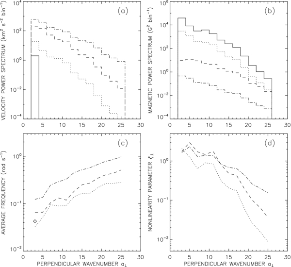
Figure 8. Power spectra and related quantities for the reference model: (a) velocity power spectra, (b) magnetic power spectra, (c) average frequency of the velocity fluctuations, (d) parameter describing the degree of nonlinearity of the waves (). These quantities are plotted as a function of the dimensionless perpendicular wavenumber a⊥. The different curves indicate different positions along the loop: photospheric base (z = 0, solid curves, diamond), temperature minimum region (z = 0.50 Mm, dotted curves), chromosphere (z = 1.52 Mm, dashed curves), corona (z = 25.2 Mm, dash-dotted curves).


Download figure:
Standard image High-resolution imageFor each wave mode k and height z, we can also determine the temporal power spectrum of the velocity fluctuations. Here is the wave frequency in radians per second. We compute this power spectrum by taking the Fourier Transform of the velocity stream function fk(z, t) with respect to time, and then multiplying the result by the square of the perpendicular wavenumber, k⊥ = ak/R(z). The average frequency of the waves can be defined as an average over the power spectrum:


We further average these frequencies over modes k to obtain the average frequency for each bin n in wavenumber space. The three curves in Figure 8(c) show for three different heights in the reference model. Note that these average frequencies generally increase with perpendicular wavenumber, as expected for turbulent flows. The diamond symbol in Figure 8(c) indicates the average frequency of the footpoint motions.


In fully developed Alfvénic turbulence, the fluctuation are expected to reach a “critical balance” in which the average wave period is of the order of the nonlinear transfer time, (k⊥v⊥)−1, where v⊥ is the average velocity. Following Goldreich & Sridhar (1995), we define a nonlinearity parameter

where v⊥, n is the average velocity based on the power in bin n, which is given by v2⊥, n = PV, na⊥, n/Δa. Figure 8(d) shows ζn as a function of dimensionless perpendicular wavenumber. Note that for low wavenumbers ζn ∼ 1, indicating the presence of strong turbulence at all heights. At large wavenumbers ζn drops below unity, which is due to wave damping.
These figures demonstrate that the waves injected into the corona through the TR have a broad range of perpendicular wavenumbers and have temporal frequencies that are very different from the driver modes launched at the base of the photosphere. Therefore, the dynamics of waves and turbulence in the lower atmosphere is very important for understanding the coronal heating problem.
4.3. Open Field Model
To demonstrate that the turbulence in the lower atmosphere is nearly independent of processes in the corona, we construct an open field model with the tube connected to the photosphere only at one end. In this model there is only a single TR, and the coronal part of the tube has constant temperature, density, and field strength (T0 = 1.5 MK, ρ0 = 9 × 10⁻¹⁵ g cm−3, Bcor = 50 G). At the coronal end of the tube we use open boundary conditions such that the Alfvén waves propagate out of the computational domain and no waves are injected. In the coronal part of this model there are only outward propagating waves, hence no nonlinear wave–wave interactions. However, wave reflection still occurs in the chromosphere and TR, so there are counter-propagating waves in the lower atmosphere, which generates strong turbulence. In Figure 9, various quantities are plotted as a function of position along the flux tube for this open field model. Comparison of Figures 5 and 9 indicates that the energy density, heating rate, and other parameters of the turbulence in the lower atmosphere (τ < 81.3 s) are very similar to those in the closed field model. Figure 9(d) shows that the corona (region with τ > 81.3 s) is still being heated, but this residual heating is due to the damping of the outward traveling waves, and is not due to turbulence.
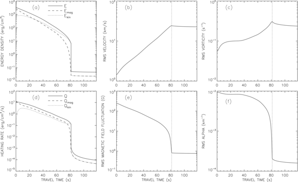
Figure 9. Model for Alfvén wave turbulence in an open field. Various quantities are plotted as a function of position along the flux tube: (a) kinetic and magnetic energy densities, and their sum E(z); (b) rms velocity Δvrms; (c) rms vorticity ωrms; (d) kinetic and magnetic heating rates, and their sum Q(z); (e) rms magnetic fluctuation ΔBrms; and (f) rms twist parameter αrms. Positions are given in terms of the Alfvén travel time τ(z). The corona is located in the range 81.3 s < τ < 118.6 s. The TR is indicated by the vertical dotted line.
Download figure:
Standard image High-resolution imageIn the above simplified model for the open field, there is no turbulent decay of the Alfvén waves in the corona. However, more realistic models of coronal holes and other open-field structures have shown that there is significant reflection of waves in the corona, and that Alfvén wave turbulence can explain the heating and acceleration of the solar wind (e.g., Dmitruk et al. 2002; Cranmer & van Ballegooijen 2005; Cranmer et al. 2007; Chandran & Hollweg 2009; Verdini et al. 2010).
4.4. Dependence of Heating Rate on Model Parameters
We construct a series of closed field models with different values of the model parameters. Table 1 shows the subset of models in which the properties of the footpoint motions or the coronal loop length are varied. The first five columns in Table 1 show the model name, the correlation time τ0, vorticity ω0 and velocity Δvrms of the footpoint motions, and the loop length Lcor. Model 21 is the reference model described in the previous subsection, and models 22–27 are variants in which one of the parameters τ0, ω0, or Lcor is changed relative to the reference model. For all models listed in Table 1, the coronal field strength Bcor = 50 G, the height of the transition region zTR = 1.8 Mm, the coronal pressure pcor = 1.833 dyne cm−2, the time step Δt0 = 0.746 s, the expansion factor Γ = 1, and damping rate νmax = 0.7 s−1.
Table 1. Dependence of Heating Rates on Footpoint Motions and Coronal Loop Length
| Model | τ0 | ω0 | Δvrms | Lcor | η | Qchrom | Qcor |
|---|---|---|---|---|---|---|---|
| (s) | (s−1) | (km s−1) | (Mm) | (erg s−1 cm−3) | (erg s−1 cm−3) | ||
| 21 | 60 | 0.04 | 1.48 | 49.6 | 0.346 | 6.08 × 10⁻¹ | 2.97 × 10⁻³ |
| 22 | 100 | 0.04 | 1.48 | 49.6 | 0.399 | 6.30 × 10⁻¹ | 2.30 × 10⁻³ |
| 23 | 200 | 0.04 | 1.48 | 49.6 | 0.440 | 5.03 × 10⁻¹ | 1.89 × 10⁻³ |
| 24 | 60 | 0.02 | 0.74 | 49.6 | 0.434 | 1.29 × 10⁻¹ | 0.90 × 10⁻³ |
| 25 | 60 | 0.06 | 2.21 | 49.6 | 0.350 | 1.59 × 100 | 5.46 × 10⁻³ |
| 26 | 60 | 0.04 | 1.48 | 25.6 | 0.362 | 6.01 × 10⁻¹ | 5.23 × 10⁻³ |
| 27 | 60 | 0.04 | 1.48 | 99.6 | 0.360 | 6.47 × 10⁻¹ | 1.49 × 10⁻³ |
Download table as: ASCIITypeset image
For each model we simulate the dynamics of the Alfvén waves generated by random footpoint motions for a period of 3000 s, and we compute the heating rate Q(z) averaged over the time interval t = [800, 3000] s of the simulation. The period before t = 800 s is omitted because it sometimes contains a large spike in heating that may be an artifact of the initial conditions. The heating rate Q(z) decreases with height in the lower atmosphere. The average heating rate in the chromosphere is determined as follows. The function Q(z) in the height range z = [700, 1300] km is fit with the following expression:

where ρchrom is the density at z = 1000 km (ρchrom ≈ 3.6 × 10⁻¹¹ g cm−3), and Qchrom and η are constants, which are determined by the fit. Therefore, Qchrom is the average heating rate at height z = 1000 km. We also measure the average coronal heating rate, Qcor. The values of η, Qchrom, and Qcor are listed in the last three columns of Table 1. Based on the results in Table 1, the coronal heating rate can be approximated as

where τ0 is in seconds. Therefore, the heating rate increases nonlinearly with the vorticity ω0 of the footpoint motions, and decreases approximately inversely with loop length Lcor.
Table 2 shows the subset of models in which the coronal field strength and plasma pressure are varied. The pressure is controlled by the TR height, zTR (see Section 3.2). The first six columns in Table 2 show the model name, the coronal field strength Bcor, the TR height zTR, the coronal pressure pcor, the loop length Lcor, and the time step Δt0 used in the simulation. Lcor is listed here because it varies slightly between these models (see Appendix B). The values of coronal field strength typically found in active regions lie in the range 10–500 G. However, the present version of the RMHD code has difficulty simulating Alfvén waves in loops with Bcor > 200 G, which is due to the large Alfvén speeds involved (vA > 7000 km s−1). Therefore, in the present paper we only consider loops with Bcor in the range 12–200 G. For all models shown in Table 2, the footpoint motions are characterized by τ0 = 60 s, ω0 = 0.04 s−1, and Δvrms = 1.48 km s−1. As before, the expansion factor Γ = 1 and the damping rate νmax = 0.7 s−1. For each model we compute the heating rate Q(z) averaged over the time interval t = [800, 3000] s of the simulation, and we derive the parameters η, Qchrom, and Qcor (see the last three columns of Table 2).
Table 2. Dependence of Heating Rates on Coronal Field Strength and Plasma Pressure
| Model | Bcor | zTR | pcor | Lcor | Δt0 | η | Qchrom | Qcor |
|---|---|---|---|---|---|---|---|---|
| (G) | (Mm) | (dyne cm−2) | (Mm) | (s) | (erg s−1 cm−3) | (erg s−1 cm−3) | ||
| 54 | 200 | 1.5 | 4.585 | 50.3 | 0.296 | 0.544 | 1.268 | 6.86 × 10⁻³ |
| 52 | 200 | 1.6 | 3.375 | 50.4 | 0.252 | 0.514 | 1.357 | 6.76 × 10⁻³ |
| 53 | 200 | 1.7 | 2.487 | 50.6 | 0.216 | 0.496 | 1.386 | 6.47 × 10⁻³ |
| 51 | 200 | 1.8 | 1.833 | 49.4 | 0.186 | 0.544 | 1.236 | 5.43 × 10⁻³ |
| 55 | 150 | 1.5 | 4.585 | 50.0 | 0.392 | 0.501 | 1.062 | 5.07 × 10⁻³ |
| 56 | 150 | 1.6 | 3.375 | 50.5 | 0.337 | 0.475 | 1.144 | 5.12 × 10⁻³ |
| 57 | 150 | 1.7 | 2.487 | 49.4 | 0.289 | 0.489 | 1.099 | 4.84 × 10⁻³ |
| 58 | 150 | 1.8 | 1.833 | 50.6 | 0.247 | 0.483 | 1.017 | 4.61 × 10⁻³ |
| 38 | 100 | 1.6 | 3.375 | 50.6 | 0.507 | 0.427 | 7.89 × 10⁻¹ | 3.75 × 10⁻³ |
| 44 | 100 | 1.7 | 2.487 | 50.7 | 0.433 | 0.425 | 8.05 × 10⁻¹ | 3.76 × 10⁻³ |
| 29 | 100 | 1.8 | 1.833 | 49.5 | 0.373 | 0.436 | 8.19 × 10⁻¹ | 3.42 × 10⁻³ |
| 42 | 100 | 1.9 | 1.351 | 49.5 | 0.319 | 0.440 | 8.00 × 10⁻¹ | 3.36 × 10⁻³ |
| 40 | 100 | 2.0 | 0.996 | 50.5 | 0.274 | 0.431 | 8.06 × 10⁻¹ | 3.03 × 10⁻³ |
| 36 | 100 | 2.1 | 0.734 | 50.1 | 0.235 | 0.442 | 8.03 × 10⁻¹ | 2.66 × 10⁻³ |
| 30 | 50 | 1.6 | 3.375 | 49.3 | 1.016 | 0.405 | 5.63 × 10⁻¹ | 2.90 × 10⁻³ |
| 32 | 50 | 1.7 | 2.487 | 50.5 | 0.864 | 0.392 | 5.99 × 10⁻¹ | 2.93 × 10⁻³ |
| 21 | 50 | 1.8 | 1.833 | 49.6 | 0.746 | 0.346 | 6.08 × 10⁻¹ | 2.97 × 10⁻³ |
| 33 | 50 | 1.9 | 1.351 | 50.5 | 0.637 | 0.392 | 5.83 × 10⁻¹ | 2.71 × 10⁻³ |
| 34 | 50 | 2.0 | 0.996 | 50.6 | 0.549 | 0.360 | 6.03 × 10⁻¹ | 2.64 × 10⁻³ |
| 31 | 50 | 2.1 | 0.734 | 50.1 | 0.469 | 0.365 | 6.01 × 10⁻¹ | 2.35 × 10⁻³ |
| 35 | 50 | 2.3 | 0.399 | 50.4 | 0.347 | 0.371 | 5.75 × 10⁻¹ | 2.06 × 10⁻³ |
| 39 | 25 | 1.6 | 3.375 | 50.4 | 2.018 | 0.423 | 4.63 × 10⁻¹ | 2.23 × 10⁻³ |
| 45 | 25 | 1.7 | 2.487 | 50.3 | 1.721 | 0.403 | 4.44 × 10⁻¹ | 2.13 × 10⁻³ |
| 28 | 25 | 1.8 | 1.833 | 49.5 | 1.481 | 0.372 | 4.61 × 10⁻¹ | 2.05 × 10⁻³ |
| 43 | 25 | 1.9 | 1.351 | 50.3 | 1.269 | 0.390 | 4.46 × 10⁻¹ | 2.05 × 10⁻³ |
| 41 | 25 | 2.0 | 0.996 | 49.5 | 1.100 | 0.407 | 4.45 × 10⁻¹ | 1.88 × 10⁻³ |
| 37 | 25 | 2.1 | 0.734 | 50.4 | 0.944 | 0.422 | 4.19 × 10⁻¹ | 1.85 × 10⁻³ |
| 46 | 25 | 2.3 | 0.399 | 50.4 | 0.694 | 0.389 | 4.31 × 10⁻¹ | 1.61 × 10⁻³ |
| 50 | 12 | 1.9 | 1.351 | 49.6 | 2.669 | 0.414 | 3.51 × 10⁻¹ | 1.39 × 10⁻³ |
| 49 | 12 | 2.0 | 0.996 | 50.5 | 2.283 | 0.406 | 3.70 × 10⁻¹ | 1.33 × 10⁻³ |
| 48 | 12 | 2.1 | 0.734 | 50.4 | 1.967 | 0.382 | 3.61 × 10⁻¹ | 1.30 × 10⁻³ |
| 47 | 12 | 2.3 | 0.399 | 50.1 | 1.438 | 0.373 | 3.52 × 10⁻¹ | 1.21 × 10⁻³ |
Download table as: ASCIITypeset image
Figures 10(a) and (b) show the coronal and chromospheric heating rates as a function of coronal pressure pcor for six values of coronal field strength (Bcor = 12, 25, 50, 100, 150, and 200 G). The symbols show the simulation data listed in Table 2, and the dashed curves show quadratic fits to these data. Both Qcor and Qchrom increase with coronal field strength. The decrease of Qcor for low coronal pressures may be explained as effects of wave reflection: for small pcor or high Bcor the coronal Alfvén speed is very high, resulting in strong wave reflection in the chromosphere and TR. As a result, a larger fraction of the wave energy is dissipated in the lower atmosphere. Figure 10(b) shows that the chromospheric heating rate depends only weakly on coronal pressure.
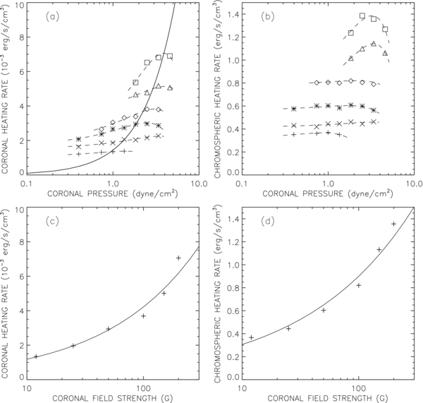
Figure 10. Dependence of coronal and chromospheric heating rates on coronal pressure (pcor) and field strength (Bcor) for a loop with constant cross section and length Lcor = 50 Mm. (a) Average coronal heating rate Qcor as a function of pcor. The symbols show results from the numerical models listed in Table 2 for Bcor = 12 G (plusses), 25 G (crosses), 50 (stars), 100 G (diamonds), 150 G (triangles), and 200 G (squares). The dashed curves show quadratic fits to these data, and the solid curve shows the heating rate predicted by the RTV scaling law, Equation (2). The latter represents the condition of thermal equilibrium (balance between heating and cooling processes). (b) Heating rate Qchrom at height z = 1 Mm in the chromosphere, plotted as a function of coronal pressure. Panels (c) and (d) show the equilibrium heating rates Qcor and Qchrom as a function of coronal field strength. The plus signs show the values derived from the intersections of the dashed and solid curves in panel (a), and the solid curves show power-law fits to these data, see Equations (61) and (62).
Download figure:
Standard image High-resolution imageAs discussed in Section 3.2, the peak temperature Tmax along a coronal loop was chosen to be consistent with the first RTV scaling law, Equation (1), but the heating rates Qcor found in the simulations are not necessarily consistent with the second scaling law, Equation (2). Therefore, the models listed in Tables 1 and 2 are not necessarily in thermal equilibrium. The solid curve in Figure 10(a) shows the heating rate Qcor derived from Equation (2) with Lcor = 50 Mm. This curve shows the value of Qcor at which the coronal loop is in thermal equilibrium (i.e., the heating is balanced by radiative and conductive losses). To the left of this curve, the time-averaged heating rate due to Alfvén wave turbulence is larger than the radiative and conductive losses, so the coronal temperature will increase, more mass will be evaporated into the corona from the chromosphere, and the coronal pressure will increase. The opposite happens to the right of the solid curve. Therefore, although the present models do not include the effects of chromospheric evaporation, it is clear that in models with time-dependent coronal pressure the corona will have a tendency to approach the equilibrium state represented by the RTV scaling laws.
The field-strength dependence of the equilibrium heating rate Qcor can be determined by finding the intersection points of the solid and dashed curves in Figure 10(a), and the corresponding chromospheric heating rate Qchrom can be obtained from Figure 10(b). The “equilibrium” heating rates are plotted in Figures 10(c) and (d) as a function of coronal field strength, Bcor. Note that both heating rates increase with coronal field strength, and show no sign of saturation for large Bcor. The dependences on Bcor can be roughly approximated as power laws:


although the fits are not very accurate at high field strength (see solid curves in Figures 10(c) and (d)). Combining Equations (60) and (61), we obtain

where we replaced the vorticity ω0 by the velocity Δvrms of the footpoint motions. Note that the equilibrium heating rate depends on coronal field strength Bcor, on loop length Lcor, and on the parameters of the footpoint motions (τ0 and Δvrms).
The above expression assumes that the coronal temperature and pressure have the values predicted by the RTV scaling laws, and therefore neglects the effects of the spatial and temporal variability of the heating (Klimchuk 2006). Also, it should be kept in mind that the numerical simulations have been done only in a limited range of coronal field strength and loop length (12 G < Bcor < 200 G, 25 Mm < Lcor < 100 Mm), so the above expression for Qcor is valid only within this limited range. Furthermore, the above expression applies only to coronal loops with constant cross section (Γ = 1), and the effects of gravity have been neglected in the corona (but not in the lower atmosphere). Expression (63) should not be applied to coronal loops on the quiet Sun, where magnetic fields are weaker and the effects of gravity and coronal loop expansion cannot be neglected.
We also considered how the heating rates depend on the maximum damping rate νmax of the Alfvén modes (see Equation (B13)). For model nos. 21, 28, and 29 we did a second simulation with twice the damping rate (νmax = 1.4 s−1), and we found that the coronal heating rates Qcor are changed by about +1%, −6%, and −6%, respectively. The chromospheric heating rates Qchrom are changed by −6%, +2%, and −10% for these three models. These numbers are relatively small compared to the factor two change in the damping rate, indicating that the rate of turbulent dissipation is insensitive to the value of the damping rate of the high wavenumber modes, as one would expect for a turbulent process.
4.5. Effects of Coronal Loop Expansion
Models of the coronal magnetic field (e.g., Schrijver et al. 2005) predict that the field strength B0 generally decreases with height in the corona. Therefore, we expect that the cross-sectional area A of a coronal loop increases with height: A = Φ/B0, where Φ is the magnetic flux, which presumably is constant along the loop. However, observed X-ray and EUV loops often show approximately constant cross section (Klimchuk 2000; Watko & Klimchuk 2000; López Fuentes et al. 2006). The reasons for this discrepancy are not well understood. The present paper cannot directly address this issue because our model does not include interactions between neighboring flux tubes, which we believe is important for resolving this issue. However, we can investigate how Alfvén waves are affected by the expansion of the loop with height. We define the areal expansion factor Γ as described in Equation (51). This factor affects only the coronal part of the loop and has no effect on the magnetic field B0(z) in the lower atmosphere. We construct a series of models with different expansion factors, but otherwise identical model parameters (zTR = 1.8 Mm, Lcor = 50 Mm, Bcor = 50 G). For each model we compute the heating rate per unit volume, Q(z), averaged over the time interval from 800 to 3000 s and over the cross-sectional area of the flux tube. We also compute the rate of energy input into the corona,

where A(z) = πR2(z) is the cross-sectional area of the tube, zTR1 and zTR2 are the positions of the TRs, and FA(z) is the time-averaged Alfvén wave energy flux (see Equation (C12)). Finally, we compute two energy dissipation rates, Ptot and Pcor, which represent the dissipated power integrated over the total volume of the tube and over the coronal volume, respectively:

We find that Pcor and P′cor are equal to within a few percent, as expected for a statistically stationary state. This equality also shows that energy is very well conserved in these numerical models.
The results of the simulations are summarized in Table 3. The nine columns of this table show the areal expansion factor Γ, the coronal volume Vcor, the parameters η, and Qchrom describing the heating in the lower atmosphere (see Equation (59)), the volume-averaged coronal heating rate Qcor, the Alfvén wave energy flux FA(zTR) at the TR, the integrated dissipation rates Ptot and Pcor, and the fraction of energy dissipated in the corona, fcor ≡ Pcor/Ptot. The model with Γ = 1 is the reference model discussed in Section 4.1. We find that for the reference model only 7.7% of the available energy is dissipated in the corona; the remainder is dissipated in the photosphere and chromosphere at the two ends of the coronal loop. The energy flux FA(zTR) increases with the expansion factor, and so does the coronal power Pcor and the fraction fcor. Specifically, for Γ = 6 about 16% of the available energy is dissipated in the corona. In contrast, the total dissipation rate Ptot is almost independent of the expansion factor. Therefore, the heating of the lower atmosphere is apparently not sensitive to the properties of the coronal part of the loop.
Table 3. Effect of Coronal Loop Expansion.
| Γ | Vcor | η | Qchrom | Qcor | FA(zTR) | Ptot | Pcor | fcor |
|---|---|---|---|---|---|---|---|---|
| (cm−3) | (erg s−1 cm−3) | (erg s−1 cm−3) | () | (erg s−1) | (erg s−1) | |||
| 1 | 0.44 × 1026 | 0.346 | 6.08 × 10⁻¹ | 2.97 × 10⁻³ | 0.77 × 10⁷ | 1.69 × 1024 | 1.30 × 10²³ | 0.077 |
| 2 | 0.73 × 1026 | 0.386 | 5.70 × 10⁻¹ | 2.54 × 10⁻³ | 1.09 × 10⁷ | 1.66 × 1024 | 1.85 × 10²³ | 0.111 |
| 3 | 1.03 × 1026 | 0.353 | 5.57 × 10⁻¹ | 2.11 × 10⁻³ | 1.25 × 10⁷ | 1.66 × 1024 | 2.17 × 10²³ | 0.130 |
| 4 | 1.32 × 1026 | 0.377 | 5.75 × 10⁻¹ | 1.76 × 10⁻³ | 1.34 × 10⁷ | 1.70 × 1024 | 2.32 × 10²³ | 0.137 |
| 6 | 1.91 × 1026 | 0.371 | 5.53 × 10⁻¹ | 1.43 × 10⁻³ | 1.56 × 10⁷ | 1.69 × 1024 | 2.73 × 10²³ | 0.161 |

Download table as: ASCIITypeset image
The results of Table 3 show that, as Γ increases, more energy enters into the corona and is dissipated at coronal heights. We suggest this increase is due to the fact that for large Γ the Alfvén speed at the midpoint of the coronal loop (z = L/2) is drastically reduced compared to the case Γ = 1. As a result, it takes a longer time for the Alfvén waves to travel through the corona, and this gives the waves more time to dissipate their energy in the corona via turbulent processes. The wave energy is distributed over a coronal volume Vcor that increases more rapidly with Γ than the energy dissipation rate. Therefore, the average heating rate Qcor in the corona decreases with increasing Γ (see Table 3).
Figure 11 shows the magnetic field strength B0(z) and time-averaged volumetric heating rate Q(z) as functions of position along the coronal loop. Note that Q(z) is relatively constant within the corona and varies more gradually than the magnetic field strength B0(z). A power-law fit to these data for Γ = 4 and 6 yields Q(z)∝[B0(z)]0.4, so the exponent is significantly less than unity. We suggest that this relative constancy of the volumetric heating rate may be due to Alfvén wave reflection within the corona. For large Γ, the Alfvén speed vA(z) has a local minimum at the mid-point of the loop (z = 27 Mm), and increases toward the ends. Hence, as the Alfvén waves travel from the midpoint to the ends of the loop, the waves are partially reflected before they reach the TR. This enhances the wave energy density in the central part of the loop and gives the wave more time to be dissipated near the midpoint. Clearly, wave reflections in the chromosphere, at the TR, and within the corona play an important role in determining the spatial distribution of the average heating rate Q(z).

Figure 11. Effects of coronal loop expansion. (a) Magnetic field strength B0(z) and (b) volumetric heating rate Q(z), as functions of position z along the coronal loop for different values of the loop expansion factor: Γ = 1 (full), Γ = 2 (dotted), Γ = 3 (dashed), Γ = 4 (dash-dotted), and Γ = 6 (triple-dot-dashed).
Download figure:
Standard image High-resolution imageIt is worthwhile to compare the computed heating rates Q(z) with those predicted from phenomenological turbulence models (Hossain et al. 1995; Matthaeus et al. 1999; Dmitruk et al. 2001, 2002; Chandran et al. 2009). In such models the fluctuations are expressed in terms of the Elsasser variables, here defined as . The turbulent dissipation rate is given by Equation (57) of Cranmer & van Ballegooijen (2005):


where L⊥(z) is the outer scale of the turbulence and the quantities Z±(z) are the rms values of the Elsasser variables. The latter are averaged over the cross section of the flux tube (see Equation (C3)) and over time. We compute Z±(z) for several models and find that the turbulence is significantly unbalanced (Z+ ≠ Z−), which is due to the strong dissipation in our models. The perpendicular length scale is set equal to the flux tube radius, L⊥ = R(z). Figure 12 shows the ratio q(z) ≡ Q(z)/Qphen(z) plotted as a function of position along the flux tube for three values of the coronal loop expansion factor (Γ = 1, 3, and 6). Positions are given in terms of the Alfvén travel time τ(z) from the left footpoint. We find that q ≈ 0.2 in the photosphere and low chromosphere, and the ratio peaks in the upper chromosphere, indicating the turbulence is more efficient there. For the reference model q ≈ 0.3 in the corona (solid curve), similar to the value of 0.5 used by Breech et al. (2009) in their model of the solar wind. Similar values for q are found for the models with larger expansion factors (the downward spikes just above the TR may be due to insufficient spatial resolution). We conclude that q is significantly less than unity at all heights.
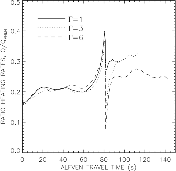
Figure 12. Ratio of the numerically computed heating rate Q(z) and the rate Qphen(z) predicted by phenomenological turbulence models. The ratio q ≡ Q/Qphen is plotted as a function of Alfvén travel time τ(z) from the left footpoint for three different values of the loop expansion factor: Γ = 1 (full), Γ = 3 (dotted), and Γ = 6 (dashed). Only half of the loop is shown (0 < z < L/2).
Download figure:
Standard image High-resolution image5. SUMMARY AND DISCUSSION
According to the present model, the interactions of turbulent convective flows with kilogauss flux tubes in the photosphere produce transverse displacements of magnetic field lines on length scales less than the width of the flux tubes, i.e., less than about 100 km (see Figure 1). We assumed that the photospheric footpoint motions have velocity amplitudes in the range 1–2 km s−1 and correlation times of 60–200 s. We studied the dynamics of the Alfvén waves produced by such footpoint motions, and found that such motions produce Alfvénic turbulence at larger heights in the flux tube. The predicted dissipation rates of the turbulence as a function of height are sufficient to reproduce the observed rates of chromospheric and coronal heating in active regions. We conclude that fine scale magnetic braiding can drive Alfvénic turbulence and can produce sufficient heating for both the chromosphere and corona. However, we should emphasize that we do not have any direct observational evidence for the existence of the assumed footpoint motions, as scales of 100 km or less cannot be resolved with present-day solar telescopes. Therefore, our conclusion can be made only for the chosen values of the photospheric driver; for higher or lower values the heating does not meet the observational constraints. Our results indirectly provide a constraint on the amplitude of the footpoint motions necessary for the proposed mechanism to heat the chromosphere and corona. Our model produces a coronal heating profile that is similar to that of a nanoflare storm (Klimchuk 2006) in the spatial and temporal distribution of heating events, and in the final source of the energy released—dissipation of magnetic fields. The difference is that we have provided a fully self-consistent source for the nanoflare energy. The source depends critically on the existence of a chromospheric reservoir of turbulent Alfvén waves.
To investigate the nonlinear dynamics of the Alfvén waves, we considered a flux tube that extends from the photosphere through the chromosphere into the corona. We mainly considered closed coronal loops, and for simplicity we assumed that a single kilogauss flux tube at one end of the loop is connected to a single flux tube at the other end. Therefore, we ignored the fact that on the real Sun the photospheric flux concentrations at the two ends are uncorrelated and do not perfectly match up. Furthermore, we assumed that the flux elements do not split up or merge during the simulation, so that the flux tube retains its identity. The pressure, density, and magnetic field strength were taken to be fixed functions of position z along the flux tube. The assumed structure of the lower atmosphere is based on model P by Fontenla et al. (2009); this model represents faculae in active regions (i.e., very bright plage). The chromosphere–corona TR was treated as a discontinuity where waves can reflect, and we neglected the gravitational stratification in the corona, so the pressure is constant along the coronal part of the loop.
The dynamics of the waves and their structure in the plane perpendicular to the loop axis were described using the RMHD approximation (Strauss 1976), which assumes that the magnetic and velocity perturbations of the waves are perpendicular to the mean magnetic field of the flux tube. We found that the Alfvén waves strongly reflect as they propagate through the chromosphere. This reflection is due to the increase of Alfvén speed with height. Even stronger reflection occurs at the TR where the Alfvén speed suddenly increases by about a factor of 15. These reflections produce in the chromosphere a pattern of counter-propagating waves that are subject to nonlinear wave–wave interactions. We found that the waves quickly decay into turbulence, causing most of the wave energy to be deposited in the lower atmosphere (photosphere and chromosphere). Only a small fraction of the wave energy is transmitted into the corona. Energy is injected at both ends of the coronal loop, producing in the corona two sets of counter-propagating waves that reflect off the TRs and decay into turbulence. The dissipation is entirely due to Alfvén wave turbulence and is not due to phase mixing or resonant absorption (e.g., Heyvaerts & Priest 1983; De Groof & Goossens 2002), which are not included in the present model.
We constructed a variety of loop models with different values of the model parameters. For the reference model (Section 4.1) we assumed the photospheric footpoint motions have an rms velocity of 1.48 km s−1 and a correlation time τ0 = 60 s. We found that the heating rate Q(z, t) varies strongly with position z along the loop and with time, which is due to bursts of wave activity and subsequent dissipation of the waves via turbulence. Only a small fraction of the wave energy is dissipated in the corona (about 7.7%), and the remainder is dissipated in the lower atmospheres at the two ends of the modeled loop. We computed the time-averaged heating rate Q(z) and found that this rate decreases with height in the lower atmosphere from about 10 erg cm−3 s−1 in the photosphere to about 0.2 erg cm−3 s−1 in the upper chromosphere. These values can be compared with rates of radiative loss found in semiempirical models of the solar atmosphere (e.g., Avrett 1985; Anderson & Athay 1989; Fontenla et al. 1999, 2006, 2009). Fontenla et al. (2009) computed radiative loss rates as a function of gas pressure (i.e., height) for several different wavelength bands (see their Figure 14). For model P the largest radiative loss occurs in the 2000–3000 Å band, which contains the Mg ii resonance lines. The total losses over all wavelengths are in the range 1–2 erg cm−3 s−1, somewhat larger than the values found in the present model. Therefore, our model may underestimate the amplitude of the Alfvén waves and rate of energy dissipation in the chromosphere.
In the corona the reference model predicts Qcor ∼ 3 × 10⁻³ erg cm−3 s−1, which is sufficient to explain the heating of typical active region loops. The predicted velocity amplitude of the Alfvén waves in the corona is in the range 20–40 km s−1, similar to the values found in observations of spectral line widths in active regions (Dere & Mason 1993; Warren et al. 2008; Li & Ding 2009). We investigated how the coronal and chromospheric heating rates depend on the model parameters (see Section 4.4). We used the RTV scaling laws to determine the “equilibrium” heating rates for which the coronal heating is balanced by radiative and conductive losses, and derived a scaling law describing how the coronal heating rate Qcor depends on the coronal field strength, loop length, and the parameters of the footpoint motions (Equation (63)). This result may be compared with other models of coronal heating (see Mandrini et al. 2000; Schrijver et al. 2004).
We also considered coronal loops with non-constant cross section (Section 4.5) and found that both the energy flux FA(zTR) entering the corona and the total power Pcor dissipated in the corona increases with the areal expansion factor Γ. The increase of Pcor with Γ is due to the decrease in the coronal Alfvén speed, which lengthens the Alfvén travel time in the corona and gives the waves more time to dissipate their energy via turbulence. The fraction of energy dissipated in the corona also increases with Γ, but is still only about 16% for the model with Γ = 6. The average coronal heating rate Qcor decreases with Γ, which is due to the fact that the coronal volume increases faster than the dissipated power Pcor. We found that for models with Γ > 1 the heating rate Q(z) varies with position along the coronal part of the loop, and decreases toward the midpoint of the loop where the field strength B0(z) is lowest. However, Q(z) varies less than B0(z), so the heating is not strongly concentrated near the coronal base. This effect can be understood in terms of reflection of the waves by gradients of Alfvén speed in the corona.
Observations of the active corona using the TRACE (see Handy et al. 1999) have shown that the corona is highly dynamic and full of flows and wave phenomena (e.g., Schrijver et al. 1999). This has led some authors to suggest that the heating of active region loops is localized in the low corona and involves energization processes that operate in the chromosphere and TR (Aschwanden 2001; Aschwanden et al. 2007; De Pontieu et al. 2009). However, Klimchuk et al. (2010) show that the heating concentrated in the low corona would lead to thermal non-equilibrium of the plasma, and such non-equilibrium is not consistent with the observed properties of warm (1–2 MK) loops observed in active regions. Instead, they suggest coronal loops are heated impulsively by storms of nanoflares that are distributed throughout the coronal loop (also see Parker 1988; Lu & Hamilton 1991; Klimchuk 2006, 2009). The present model has some features in common with both types of models. On the one hand, we find that the average heating in the chromosphere is two or three orders of magnitude larger than that in the low corona, and that most of the heating occurs in the lower atmosphere, which is consistent with the ideas of De Pontieu et al. (2009). On the other hand, in the coronal part of the loop the heating depends only weakly on position, so the loop is likely to be thermally stable, consistent with the results of Klimchuk et al. (2010).
Although the present model was described in terms of the propagation and dissipation of Alfvén waves, the waves reflect at various heights and undergo nonlinear interactions, producing twisted and braided fields similar to those found in previous braiding models (e.g., Mikić et al. 1989; Longcope & Strauss 1994; Hendrix et al. 1996; Galsgaard & Nordlund 1996; Ng & Bhattacharjee 1998; Craig & Sneyd 2005; Rappazzo et al. 2008). Also, the model includes the effects of magnetic reconnection, and the time-dependent heating seen in Figure 4(d) can be thought of as a sequence of “nanoflares” (Parker 1988). However, unlike in previous “quasi-static” braiding models the twisted structures are highly dynamic and are far from the force-free equilibrium state. For example, the twist parameter α is not at all constant along the field lines (see Figure 5(f)), as would be expected for a force-free state. This is due to the inclusion of the lower atmospheres at the two ends of the coronal loop, which produces turbulence in the chromosphere. Also, the transverse motions of field lines at the photospheric base occur entirely inside the magnetic flux elements, hence these motions do not contribute to the “random walk” of the flux elements on the photosphere. This has the advantage that the velocity amplitudes can be relatively large, yet be consistent with observational constraints on the photospheric diffusion constant (DeVore et al. 1985; Berger et al. 1998).
According to the present model, the transverse scale of the braids in the corona is very small, ℓ⊥ < Rcor = 529 km, so the braids would likely not be observable with existing X-ray or EUV telescopes. Furthermore, the rms value of the transverse field fluctuations is small compared to the mean field, ΔBrms/B0 ≈ 0.025, so the misalignment angle between the field lines and the tube axis is only about 1 4. Both the transverse scale of the braids and the misalignment angle are consistent with the fact that no braiding is observed in the corona on scales of several arcseconds or larger (see Section 2.1). The misalignment angle is much smaller than that required in quasi-static braiding models that match the observed heating rate (Parker 1983; Priest et al. 2002). We conclude that magnetic energy is injected into the corona via a dynamic (not quasi-static) braiding process. The existence of turbulence in coronal loops may have important implications for the damping of coronal loop oscillations (Nakariakov et al. 1999; Ofman & Aschwanden 2002; Roberts 2008) and for the cross-field diffusion of electrons (Galloway et al. 2006).
In the present paper we did not consider the plasma response to the heating. In future work we will construct models of the thermal structure of coronal loops heated by Alfvén wave turbulence, including the effects of thermal conduction and radiative losses. The results will be compared with predictions from quasi-static braiding models. Another line of future research will be to investigate how the temporal fluctuations of the heating rate affect the temperature and density. Is thermal conduction strong enough to smooth out the spatial and temporal fluctuations? Ideally, such studies should take into account the nonuniformity of the temperature and density in the perpendicular plane; this may require a more complete three-dimensional MHD model. We also intend to consider the interactions between neighboring flux tubes in the lower atmosphere, including the effects of the splitting and merging of kilogauss flux tubes.
We thank the anonymous referee for many useful comments which helped to improve this paper. We also thank B. Chandran for discussions on nonlinear effects in Alfvénic turbulence. Hinode is a Japanese mission developed and launched by ISAS/JAXA, with NAOJ as domestic partner and NASA and STFC (UK) as international partners. It is operated by these agencies in cooperation with ESA and NSC (Norway). This work was supported by NASA contract NNM07AB07C (NASA Solar-B X-Ray Telescope Phase-E). This research has made use of NASA's Astrophysics Data System.
APPENDIX A: COMPARISON WITH TRANSPORT EQUATIONS BASED ON ELSASSER VARIABLES
In Section 3.1, we formulated the Alfvén wave transport equations in terms of scalar fields f, h, ω, and α. In contrast, previous works often used the Elsasser variables (Elsasser 1950), which are vector fields:

where is the velocity and B⊥ = ∇h × B0 is the perturbation of the magnetic field. To demonstrate that the present formulation of the transport equations is equivalent to that used by others, we start with Equation (21) of Zhou & Matthaeus (1990):


where is the Alfvén velocity vector, U is the outflow velocity, and P is the perturbation in the total pressure (also see Dmitruk et al. 2001; Verdini & Velli 2007; Buchlin & Velli 2007; Cranmer et al. 2007). In the present paper we neglect flows along the field lines, so we set U = 0. The terms in Equation (A2) involving VA and B0 can be simplified by using Equations (8) and (12), which yields


We now take the curl of the above equation and evaluate the component parallel to the mean magnetic field. Using Equation (12) to evaluate the derivatives of , we find


where are the vorticities associated with the Elsasser variables and is given by


Combining the linear terms in Equation (A4) and using (ω+ − ω−)/2 = vAα, we find that the above equations are identical to Equations (44) and (45). Therefore, the present formalism is equivalent to that used in previous work based on Elsasser variables.
APPENDIX B: NUMERICAL METHODS
The four quantities ω, α, h, and f are determined by Equations (33), (35), (40), and (39) derived in Section 3.1. In this appendix, we describe the numerical methods used for solving these equations. Let r be the radial distance to the tube axis (r < R(z)), φ the azimuth angle, and z the distance along the tube. It is convenient to write the stream function as f(ξ, φ, z, t), where ξ ≡ r/R is the fractional distance, and similar for h, ω, and α. Then spatial derivatives along the background field can be written as partial derivatives at constant ξ; for example, in Equation (39). In this way the vector can be eliminated from the equations.


The transverse structure of the waves is described using a spectral method. We use a finite set of basis functions Fi(ξ, φ), where index i enumerates the basis functions (i = 1, …, N). The functions are assumed to vanish at the tube wall, Fi(1, φ) = 0, consistent with our requirement that v and B are parallel to the wall. The basis functions are mutually orthogonal and are normalized such that

where δij is the Kronecker delta symbol. An arbitrary spatial distribution f(ξ, φ) can always be projected onto the basis functions by evaluating

where fi are the mode amplitudes:

In the following we assume f ≈ fproj, i.e., we suppress high spatial frequencies that are not present in the basis functions. The basis functions Fi(ξ, φ) are chosen to be the eigenmodes of the ∇2⊥ operator:

where λi is the dimensionless eigenvalue. The solutions Fi(ξ, φ) are proportional to Jm(aiξ), where m = mi is the azimuthal mode number (m ⩾ 0), Jm(x) is the Bessel function of the first kind, and ai is a zero of the Bessel function, Jm(ai) ≡ 0. The modes are ordered according to their m-values (first the m = 0 modes, then m = 1 modes, etc.), and for fixed m they are ordered according to their a-values. The non-axisymmetric modes always come in pairs, one proportional to cos (mφ), the other proportional to sin (mφ), which we count as two separate modes i and i + 1, respectively. The eigenvalues of the modes are λi = −a2i. We find all modes with ai below a prescribed maximum value, amax. For example, for amax = 20 we find N = 92 modes (6 modes with m = 0, 12 modes with m = 1, 10 modes with m = 2, etc., up to m = 15). The basis functions are shown in Figure 13.
Figure 13. Ninety-two basis functions Fi(x, y) for amax = 20. The two driver modes are shown as the seventh and eighth image of the top row.
Download figure:
Standard image High-resolution imageAs shown in Section 3.1, all nonlinear terms in the RMHD equations involve the bracket operator, defined in Equation (41). In polar coordinates this quantity can be written as

where f(r, φ) and g(r, φ) are arbitrary functions. Expanding f, g, and b in terms of basis functions, we obtain

where Mkji is the coupling matrix:

Note that Mkji is anti-symmetric with respect to i and j, and using partial integration one can show that Mkji = Mikj, where we use ∂Fi/∂φ = 0 for ξ = 0. It follows that the six matrix elements that couple any three modes i, j, and k are closely related:

To compute these elements we only need to consider the case k > j > i (the “unique” elements). The three modes must have compatible cos (mφ) or sin (mφ) dependence, and for mi > 0 we only need to consider the case mk = mj + mi. We find that for amax = 20 there are 7662 unique matrix elements.
The quantities f, h, ω, and α can be written in terms of basis functions, for example:

where fi(z, t) are the amplitudes of the different transverse modes. Inserting these expressions into Equations (40) and (39), and using expression (B6), we find


where

and we added artificial damping terms. The damping rate νk is assumed to be independent of time t and position z along the tube, but depends on the perpendicular wavenumber ak to the sixth power (“hyperdiffusion”):

where νmax is the damping rate of the highest wavenumber modes (we use νmax = 0.7 s−1). The alternative form of the dynamical equations, given by Equation (44), yields

Here we omit the nonlinear and damping terms because those terms will be evaluated directly from Equations (B10) and (B11) (see below).
In order to accurately describe the Alfvén wave propagation, we use a grid of positions zn such that the Alfvén travel time Δτ between neighboring grid points is exactly equal to the time step Δt0 of the calculation:

Here vA, n + 1/2 is the average speed between grid points n and n + 1. The Alfvén travel time from the TR to any position z in the corona is

where u(z) ≡ −1 + 2(z − zTR)/Lcor, and is defined by


Here we used Equations (50), (51), and (53), and vA(zTR) is the Alfvén speed at the coronal base, . The grid of un values is found by inverting the function . To ensure that the total Alfvén travel time through the corona is a multiple of Δt0, we make a slight adjustment to the assumed coronal loop length Lcor.


We now describe the procedure for solving Equations (B10) and (B11). Let ωk, n(t) be the vorticity for mode k at grid point n and time t, and similar for the magnetic flux function hk, n(t). To advance these quantities from time t to t′ = t + Δt0, we use operator splitting, i.e., each time step Δt0 consists of two parts. In Part 1 we compute the effects of nonlinear mode coupling and damping, and in Part 2 we determine the effects of wave propagation and reflection. For Part 1 we can omit the propagation and reflection terms, i.e., the first term on the right-hand side of Equation (B10) and the first and second terms in Equation (B11). The resulting equations no longer contain any z-derivatives, so the equations can be solved separately for each position n along the loop. For Part 1, advancing ωk, n and hk, n from time t to t′ is done using a fifth-order Runge–Kutta method (Press et al. 1992, Section 16.2). The method uses adaptive step size control, i.e., the time interval Δt0 may be broken up into two or more smaller intervals with Δt < Δt0. On the other hand, for Part 2 (wave propagation and reflection) we can omit the nonlinear terms in the equations, so we instead use the linearized form of Equation (B14), where the Elsasser-like variables ω±, k, n are computed from Equation (43). The solution of Equation (B14) for time step Δt0 can be written as

where αk, n ± 1/2 is the average value of α in between neighboring grid points. The first term in Equation (B18) describes wave propagation, and the second term describes the coupling due to gradients in Alfvén speed (gradients in the TRs are treated separately, see below). Note that step 2 can be done separately for each mode k because there is no mode coupling in the linearized equations. Therefore, in each time step Δt0 the effects of both linear and nonlinear terms in the equations are taken into account.
In our model there are two chromosphere–corona TRs, one at each end of the coronal loop. At these TRs the mass density (and therefore the Alfvén speed) changes discontinuously with position, which causes strong wave reflection. Let zTR be the position of one of these TRs. In our model there are two grid points associated with this position: z1 just below the discontinuity and z2 just above it. Let vA, 1 and vA, 2 be the Alfvén speeds at these points, and let f1, ± and f2, ± be the corresponding inward and outward propagating waves (note that vA, 1 < vA, 2 for the first TR, and vA, 1 > vA, 2 for the second one). The waves f1, + and f2, − that propagate away from the TR are assumed to be linear combinations of the waves f1, − and f2, + that propagate toward it:


where the cij's are reflection and transmission coefficients. Then the stream functions in the two regions are given by


At zTR both the velocity and the magnetic field perturbations must be continuous (see Chandrasekhar 1961), so we require f1 = f2 and h1 = h2. Moreover, these conditions must be satisfied for any value of f1, − and f2, +. It follows that the coefficients cij are given by

where c ≡ vA, 2/vA, 1 is the ratio of Alfvén speeds.
The code was tested in various ways. We studied the propagation of Alfvén wave packets in a uniform flux tube to verify that no wave dispersion occurs. We also considered nonuniform tubes and verified that energy is conserved in wave reflections. For the stratified loop we verified that the total wave energy (integrated over the entire volume of the tube) is constant in time when a wave packet is present in the initial conditions, the footpoints are held fixed, and the damping rate νmax = 0. This demonstrates that wave energy is conserved by the nonlinear interactions. For the full model we verified that the energy injected by footpoint motion minus the energy dissipated by damping equals the rate of change of the total energy to an accuracy of about 5% of the net input rate.
APPENDIX C: ENERGY EQUATION FOR ALFVÉN WAVES
We first derive expressions for the averages of vector quantities over the cross section of the flux tube. The rms velocity Δvrms(z, t) is given by

where 〈 ⋅⋅⋅〉 denotes the spatial average over the cross section of the tube. Here we used partial integration to obtain ω (=−∇2⊥f), and we used Equations (B1), (B9), and (B12). Similarly, the rms magnetic fluctuation ΔBrms(z, t) is given by

and the rms values of the Elsasser variables are

It follows from Equations (C1) and (C2) that the contributions of mode k to the velocity and magnetic power spectra are

We now derive the energy equation in the context of the present model. The kinetic and magnetic energy densities are given by


Multiplying Equation (B10) by ρ0fk and summing over k, we obtain the following equation for the kinetic energy density:

where Qkin is the rate of kinetic energy loss due to damping:

Similarly, multiplying Equation (B11) by B20/(4π)(ak/R)2hk yields an equation for the magnetic energy density:

where Qmag is the rate of magnetic energy loss:

Adding Equations (C7) and (C9) yields

where E(z, t) ≡ Ekin + Emag is the total energy density, Q(z, t) ≡ Qkin + Qmag is the total dissipation rate, B0(z) represent the diverging geometry of the background field, and FA(z, t) is the Alfvén wave energy flux averaged over the cross section of the flux tube:

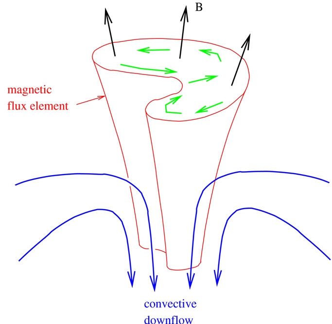
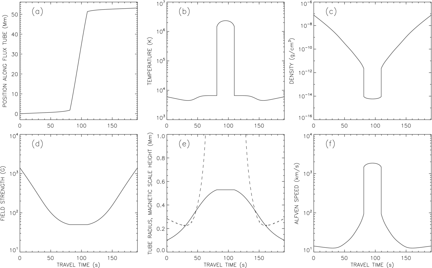
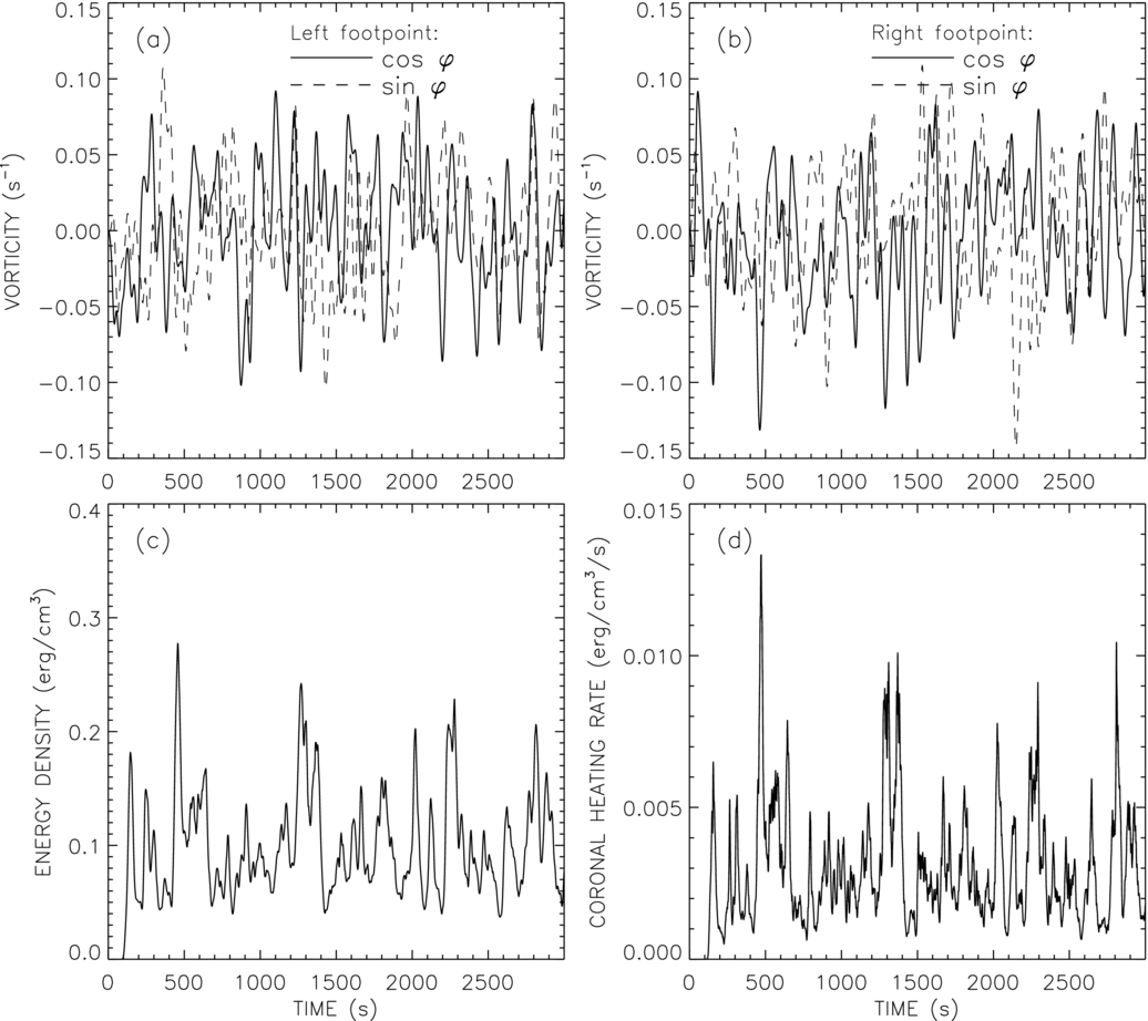
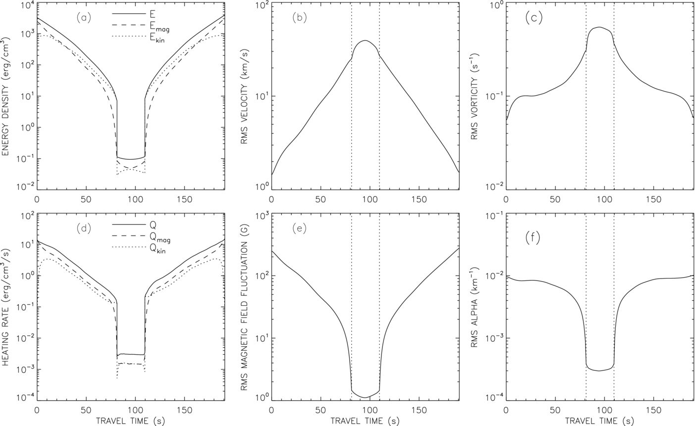
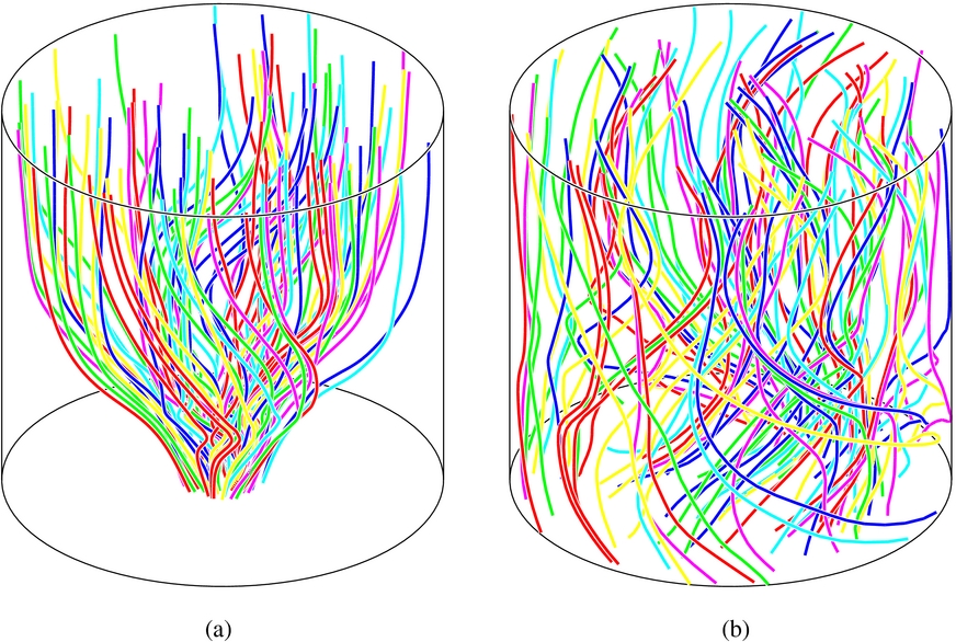
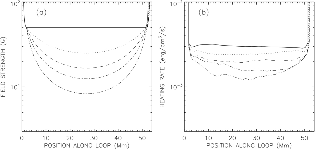
Note that the terms involving Mkji drop out of the energy equation (C11). This is a result of Equation (B8), which shows that the matrix Mkji is anti-symmetric with respect to interchange of any two indices. Therefore, the nonlinear terms in Equations (B10) and (B11) do not have a direct effect on energy transport along the tube, but they are of course responsible for exciting the high wavenumber modes that are subject to damping (Q). Therefore, our numerical scheme using basis functions Fi(ξ, φ) is excellent for studying the energetics of the waves.